The Ghost of MDX

Practically every customer over my 20+ years working with SQL Server Analysis Services (SSAS) has told me “MDX is hard to learn”. As cliche as this is to say, I think the source of difficulty is mostly that the MDX language is misunderstood. I believe that in large part, it’s because SQL and MDX are data query languages, but operate on different manifestations of data. And so the concepts within the two paradigms are incorrectly conflated.

MDX, Multi Dimensional eXpressions, is a domain-specific language for querying a multidimensional database. The notion of “multi-dimensional” matrices isn’t as readily easy to grasp as the notion of “two-dimensional” tables. Therefore, MDX is probably tougher to learn than SQL itself.

However, it’s often the case that when an underlying concept is simple, sometimes the ability to communicate advanced topics becomes really messy. Specifically, SQL is easy to pick up at beginner levels, but grows ugly at advanced levels when pushed out of its comfort zone. Simpler concepts gain traction because they are more appealing to a large audience.

Before continuing, full disclosure, I’m a Principal Solutions Architect at Kyvos Insights. The flagship product, Kyvos SmartOLAP, is a Cloud-scale OLAP system.

The objective of this blog is to demonstrate that in this Cloud era, there is still tremendous value in deploying multidimensional, pre-aggregated manifestations of data. Additionally, although I accept that SQL is the lingua franca of query languages (even SSAS and Kyvos offer a SQL alternative to MDX), I’d like to at least speak up for the elegance of MDX in relation to its ability to express analytical concepts. It’s not my intent to convince you to learn MDX – yet another language.

The big value of OLAP and MDX is that it brings data closer to the respective format and semantics for analytics. A hefty share of machine-learning is based on matrix-like structures of aggregated data. For example, linear regression, clustering, neural networks (mostly the “convolutional” part of CNN). Because of this, I believe that an MDX-like language will someday emerge (or re-emerge) to a highly receptive audience.

After relational databases clearly dominated data in the 1990s (Oracle, DB2, Informix, Sybase, then SQL Server), SQL Server Analysis Services stood out as what I think of as a NoSQL (where “No” means either “Not Only” or “No”) database before its time. But after all the NoSQL banter of the early Big Data and Cloud days, Hadoop retreated away from MapReduce to SQL, Spark did the same, GCP uses SQL, etc Instead of powering through the “great leap” (for example, when the hurdle to OOP was forced upon millions of programmers who grew up on procedural VB prior to the release of .NET) the industry backed down to the comfort zone.

I wonder if the retreat back to good ol’ SQL, has hindered the scope of thought among the general analytics population. My argument is that SQL is a domain-specific language for one-dimensional results, whereas MDX is a domain-specific language for multidimensional results. It’s just a thought that I’d like to lay out a bit in this post.

Closer to the Analysis

As illustrated in Figure 1, OLAP cubes in the tradition of SSAS and Kyvos SmartOLAP brings the data format and query semantics closer to the analytics. However, this value of pre-aggregated OLAP cubes is drowned out by the currently buzzword-inspiring capabilities of hardware and software. That is, the ability to successfully handle the transition of dauntingly massive volumes of data from ledger-like tables (CSV files, relational database tables, “one big tables”, etc) to matrix-like formats that are more conducive towards analysis.

Of course, the hardware I’m referring to are the massive data centers built by tera-sized companies such as Amazon and Microsoft composed of intricately networked commodity servers. As has been the case for decades, they again found a way to continue to simply “throw more iron at the problem”, even after Moore’s law seemed to be reaching an end.

Regarding the software aspects, I’m referring to those like Spark for handling Cloud-scale levels of data, libraries such as Python’s pandas and scipy for analysis at a fairly normal scale, and of course the very sophisticated visualization tools such as Power BI and Tableau. It’s important to note that although data visualization tools such as Power BI and Tableau mostly connect to ledger-like “table” data sources, the data is essentially contorted and presented to the user in what looks like an OLAP star-schema format.

The idea is, let the machines handle the tough translation from our ledgers (record of events) stored in the readily understood table format to the mathy form of matrices conducive to analytics needs. Let the humans request data in the easiest, seemingly most comfortable manner, freeing the humans to do other human things.

But as data volumes continue to explode and deployment of A.I. and IoT ramps up, the ability for the infrastructure to keep up with those loads will falter. As it is when the seemingly endless supply of resources runs out, such as cheap oil and cheap fresh water, we’re forced to engage methods of conservation and re-use of resources. Specifically, this means, we’ll need to rely on the ability of pre-aggregated OLAP to preserve expensive and unnecessary re-processing of massive volumes of data.

The Domain-Specific Language of Multi-Dimensional Space

As mentioned in the intro, MDX, Multi Dimensional eXpressions, is a domain-specific language for querying a multidimensional database. SQL is a domain-specific language for querying ledger-like tables.

SQL is easier to understand than MDX because SQL deals with one-dimensional constructs that are easier to comprehend than constructs with more dimensions. For example, Figure 2 shows a partial listing of sales from the AdventureWorks sales table (60,398 total rows). It’s easy to understand a ledger of sales transactions.

But wait a minute! It sure looks like the rows and columns of Figure 2 is two-dimensional? Rather, I look at it as a one-dimensional array of sales. Each row is sale; each row is just the attributes of the primary key. We just chose to separate out the elements of a sale.

In contrast to Figure 2 above, Figure 3 shows a genuinely 2-dimensional matrix of sales along two axes of customer Occupation and Education. Both Figures 2 and 3 convey the same data and are displayed in Excel.

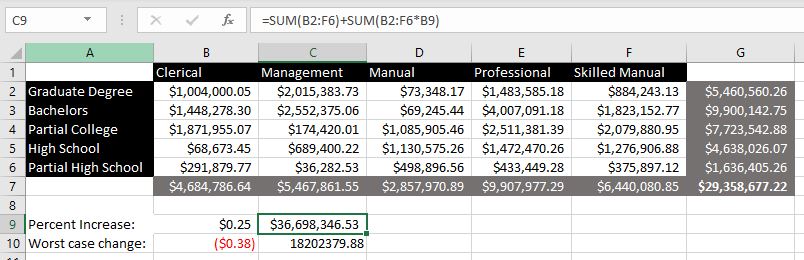
The differences between Figures 2 and 3 encapsulate much of the differences between what SQL is good for and what MDX is good for, respectively. Note that in Figure 3:

• The information that is conveyed is comprised of a very small volume of data as compared to the same data in the partial table shown in Figure 2. This is fundamental to analytics. It’s an inductive process of generalizations (a small volume of data) gleaned from massive volumes of ledger-like events.
• We’re able to perform operations (additions in this case) in all vertical and horizontal lines. The total for each line is shown in the gray boxes.
• The labels of both axes (the black boxes) are all of the same “type”. The columns are all occupation types, and the rows are all levels of education. In contrast, the columns table shown in Figure 2 are off of different types, each an attribute of a sale. Each row represents a single sale.
• The education levels are in order of the level of achievement. This conveys more information than if they were not ordinal. For example, we can see that for management roles, more education usually leads to more sales.

Of course, it’s not as if SQL isn’t capable of returning a matrix view such as that shown above in Figure 3. Figure 4a depicts the workhorse SQL GROUP BY pattern.

Figure 4b shows that SQL has become a true lingua franca in that it takes on characteristics from other languages. In this case, it’s the PIVOT function from the SQL-99 OLAP extensions. But those SQL extensions don’t address the underlying engine of a pre-aggregated OLAP. And, not all SQL dialects have implemented the SQL 99 OLAP Extensions.

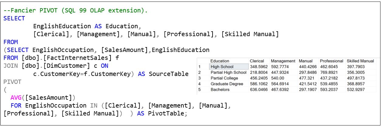
In all honesty, after over a decade of periodically composing these PIVOT/UNPIVOT SQL statements, I still struggled a bit with this one. It is a Frankenstein mess. The syntax is pretty ad-hoc to standard SQL.

The SQL shown below in Figure 5 returns the percentage change from Q4-2012 to Q4-2013 for each Education level and Gender. It’s not quite as simple as a basic SQL query to merely retrieve the sales for Customer 2000:

SELECT CustomerKey,OrderDate,SalesAmount FROM factTable WHERE CustomerKey=2000

The underlying data is the same from the AdventureWorks SQL Server database that we’ve been using from Figures 2 through 4b. However, we’ve added in common analytics function, the parallel period. In this case, comparing the sales of Q4 of this year to Q4 of last year.

There are several others ways to compose this SQL shown in Figure 5 (CTE, correlated sub query, breaking up the steps into a stored procedure, etc), but this pattern usually works best all around – for me, anyway.

Figure 6 shows the MDX retrieving the same results as what’s in Figure 5, but from the multidimensional AdventureWorks SSAS cube. Note that the values are the same, but SQL returned the values in a table-like format, whereas the MDX results are in a matrix format. That difference may seem trivial. But as Figure 3 above shows, the matrix format makes it easier to express and perform operations (addition in the case of Figure 3) across each line.

At least in the SSAS world, the result of an MDX query is an object called a cellset. Users (programmers or visualization tools) interact with that object as though it’s a matrix. This is different from the tabular result from a SQL query, whether from a pandas or Spark DataFrame or a table in a relational database. Although much of the MDX syntax shown in Figure 6 seems like arbitrary gibberish to someone who hasn’t learned MDX, the more succinct MDX might imply more elegance in the expression of this use case.

There are two reasons I think MDX is a more elegant way to query multidimensional space. Firstly, the native MDX functions encapsulate what is necessary to navigate a multidimensional structure and specify analytical calculations. That includes such goodies as navigating dimensions and hierarchies, forming sets of dimension members, and aggregating sets of tuples.

Secondly, MDX looks the same no matter how many dimensions there are in the multi-dimensional space. To help illustrate that claim, consider that most people can pick up a working knowledge of Excel within hours in large part because the method for identifying a cell value is limited to two dimensions. For example, A2 specifies the cell of the first column (A) and 2nd row (1). J21 specifies the value at the tenth column and 21st row. That’s very easy to get.

However, what if we need to specify more than two dimensions in Excel? Here are some ideas:

• 3D – Sheets, for example, Sheet1$B7
• 4D – Multiple Excel files in a directory, for example: Sheet1$B7 in customerA.xlsx
• 5D – Array of directories containing excel files, for example: Sheet1$B7 in C:\Rich_People\customerD.xlsx or C:\Poor_People\customerD.xlsx
• 6D and beyond – Hierarchy of arrays of directories. Alternatively, array of servers.

That’s not nearly as elegant a way to express a 3D tuple as with this MDX:

(

[Customer].[Education].[Graduate Degree],

[Customer].[Occupation].[Professional],

[Date].[Calendar Year].[2012],

[Sales Amount]

)

Each dimension has the same format. Dimension slices are specified with a code specifying the dimension, attribute, and finally the desired member (or members) of the attribute.

In all fairness, part of the reason 2D is enough for the general population of analysts is that it’s cumbersome to analyze a 3D visualization off a 2D monitor, and nearly impossible (at least not pragmatic) visualizing more than 3D. However, the machine learning algorithms such as K-Means, linear regression, and even convolutional neural networks can analyze in many more than three dimensions.

Data Pidgin

As mentioned, I’m not claiming MDX is “easy” to learn. The irony is that much of the wall around learning MDX is based on the fact that it looks like SQL. One of the worst design choices ever made was to decide to make it look like SQL because it would be “familiar” to database people (developers, DBAs) who would be the logical early adopters. The paradigms are too different.

With that said, though, a similar line of thought worked out well for MDX’s language counterpart in SSAS Tabular, DAX. DAX looks like the Excel functions that analysts have grown up with over a few decades.

However, I don’t think MDX is tougher to learn than say, Python. Millions of people, from complete newbies to seasoned programmers, have successfully built skills ranging from “Stackoverflow cut/paste programming” to supreme Pythonic masters. The beauty of Python is for folks at all levels to find a way to successfully use it. There are some very useful things one could do with minimal Python skill. But that goes for any skill – well, maybe with the exception of C++.

Lastly, it’s interesting to note another language that comes to mind around the context of this blog is Cypher, the language developed by Neo4j for querying their graph database. Like MDX, it’s a domain-specific language, but for querying graph databases. It too is very un-SQL. Graph databases are on the other end of the spectrum from pre-aggregated OLAP databases.

Along those lines, I’m thinking about the awful SQL extension to T-SQL supporting the graph database features cobbled onto SQL Server a few years back (I believe SQL Server 2017?). I’m thoroughly productive using Neo4j/Cypher, but struggle with the jumble of graph database stuff lobbed onto T-SQL. This is unlike how MSFT originally keeping OLAP and OLTP separate back in 1998 when SSAS originally launched (SQL Server 7.0).

Coming Up: An MDX Primer

I realize there are many questions that could be asked or challenges made based on details I haven’t yet dived into. But I didn’t want to confuse this initial message that pre-aggregated OLAP cubes and the MDX language bring the data closer to the format preferred by most analytics techniques. If I did address everything thoroughly here, it would be a very long post, just like my prior one. And none of us want that … hahaha.

Therefore, I will follow up this blog with an MDX primer to address those issues. It will explain a few key concepts I glossed over in this post that I hope will further clear up some of the misunderstanding surrounding MDX. Some of those key concepts involve very technical internals of the OLAP engines. The thing about OLAP is that it is about query performance, so it’s difficult to separate composition of MDX from the workings of the OLAP engine.