This is a sneak peek of my upcoming book, Time Molecules: The BI Side of Process Mining and Systems Thinking—to be published in the May-June 2025 timeframe.
I’ve long been fascinated by systems thinking, ever since reading The Fifth Discipline, Peter Senge, when it was first released. The idea that complex systems behave in ways that aren’t obvious from their individual parts—emergent behaviors, feedback loops, reinforcing and balancing forces—was a major shift in how I saw the world. Systems thinking provides a rich paradigm of thought, revealing how processes, not just discrete events, shape reality.
More recently, process mining has emerged as a discipline focused on reconstructing real-world processes from event data. It has advanced significantly since I first considered writing Time Molecules back in 2021, yet even now, when I ask my colleagues about it, most still don’t know what it is. While process mining has gained traction in specialized circles, it still seems quite esoteric, its full implications—especially in the BI realm—are still unfolding.
My new book complements a solid BI foundation with process mining and systems thinking. Time Molecules extends process mining into the BI world, where decision-makers have long relied on OLAP cubes to aggregate structured data for a user-friendly and highly performant query experience. But instead of pre-aggregating sums and counts across millions to trillions of transactions, Time Molecules aggregates millions to trillions of events into compressed representations known as hidden Markov models (HMM)—Markov models at scale (combined with the Tuple Correlation Web described in Enterprise Intelligence).
What is Business Intelligence?
For those unfamiliar with what I call “traditional BI,” it refers to the structured analysis of data using tools like Tableau, Power BI, Cognos, Pyramid Analytics, Qlik, and even Excel—the OG of BI tools. Those users usually have “analyst” or “manager” in their title—back when analytics was still considered a “nice to have”, not mission-critical, and unavailable to the vast majority of information/knowledge workers. That’s not the case today in this LLM-driven era of AI, where everyone should be a BI consumer.
Data is extracted from operational systems like Salesforce, SAP, or Workday, transformed into a set of consistent, business-friendly codes, and loaded into a data warehouse or data mart. From there, it may be shaped into an OLAP cube (today, a highly performant semantic model such as Kyvos) enabling fast performance and intuitive, interactive reports designed for business users—not just data professionals.
Here is a list of a few blogs of mine from my Kyvos Insights blog page that provide background into that “traditional BI”:
- All Roads Lead to OLAP Cubes … Eventually – What is the profound value of OLAP cubes?
- The Need for OLAP in the Cloud – This blog describes why OLAP cubes—particularly the Semantic Layer offered by Kyvos Insights— is still very much relevant in this post-Big Data era.
- SSAS MD to Kyvos Migration -For those who are familiar with SQL Server Analysis Services, the dominant OLAP platform during the 2000s and into the early 2010s. It provides a general introduction to Kyvos.
- Embracing Change with a Wide Breadth of Generalized Events – This is a pre-ChatGPT (published in Sept 2022, ChatGPT took off Nov 2022) pitch for Kyvos OLAP cubes in the world of event processing.
Why Hidden Markov Models?
You might be wondering why I chose Markov models over what are obviously more advanced models such as neural networks or other sequential algorithms like ARIMA or LSTMs. The reason is that Markov models are computationally lightweight—O(n)—requiring just one pass through what could be billions to trillions of rows of event data. They’re not only relatively light to compute, but also easy to cache, easy to study across dimensions, and their transition probabilities are transparent—ideal for BI workflows where fast results and interpretability matter. Sequence models like LSTMs or Transformers, or even well-established algorithms like ARIMA, while powerful, involve too much complexity for ad-hoc creation at typical OLAP scale and lack the transparency needed when the goal is structured, scalable analysis grounded in real-world processes.
However, I have written more on neural networks in another interesting context—embedded in knowledge graphs towards the goal of providing a richer “description” than could be supplied by Unicode characters alone. I strongly encourage you to read my blog, Embedding Machine Learning Models into Knowledge Graphs, after this one.
Figure 1 is an example of an HMM—a Markov model for calculating the probability of the result of a Holter Monitor test, and conditional probability of receiving a pacemaker implant given the result of the Holter Monitor. Note that the values are made up.
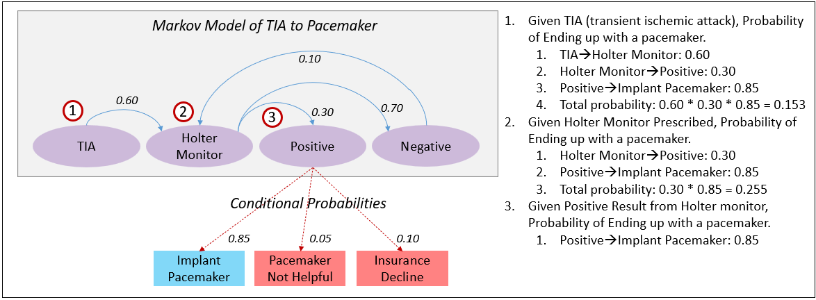
Other than the two paths outlined in Figure 1 branching from “Positive”:
- The paths leading to “Pacemaker Not Helpful” might reflect cases where a pacemaker wouldn’t be appropriate—perhaps due to high surgical risk or prior implant rejection.
- “Insurance Decline” might represent cases where insurance coverage is denied, whether due to alternative treatment recommendations, cost barriers, or the insurer deeming the procedure unnecessary or non-beneficial.
Time Molecules are a massively large collection of probabilistic HMMs across a highly multi-dimensional space—just like OLAP (Online Analytical Processing) cubes. Both optimize fundamental query patterns. OLAP cubes pre-aggregate metrics to support the classic “slice and dice” pattern—answering questions like total guitar sales in Boise in 2024. Time Molecules, on the other hand, aggregate event sequences into a compact form, supporting, “What happens next?” or “Given Event A, what’s the probability of Event B?”
HMMs are a richer structure, the underlying “DNA” of a process, encoding the likelihood of transitions rather than just an aggregated result. But I reiterate, it’s not better than the tuple-based values of traditional OLAP—it’s a complement just like particles vs. waves, space vs. time, heads vs. tails. I’m a BI architect “by trade”, so what I introduce here comes from a BI point of view. My BI roots date all the way back to my developer role on the SQL Server Analysis Services product team way back in 1998-1999.
Traditional BI asks what happened? That is, totals, averages, sums, simple calculations. Granted, OLAP can return sets (arrays) of tuples, whereby the tuples are arranged into graphic patterns we view through BI visualization tools such as Power BI and Tableau. With Time Molecules, we can query into how and why things could have happened.
But before discussing this sneak peek, I need to first back up a bit to provide some background/context—OLAP cubes. The reason is that I see Time Molecules as the time-oriented counterpart to metric-oriented OLAP cubes—the “other side of the BI coin” of high-performance and user-friendliness.
As AI-driven automation, IoT devices, and increasingly granular transaction systems generate an ever-growing stream of events, the sheer volume of analytically valuable data will exceed the comfort level of current hardware environments (very expensive SMP servers 20 years ago, datacenters today). At that point, optimization becomes non-negotiable. It becomes necessary to implement very clever optimization techniques. Time Molecules aim to do for processes what OLAP cubes did for metrics: pre-aggregate intelligently, so scale and speed coexist.
OLAP Cubes—Pre-Aggregated Structures for Fast Analysis
Knowledge is cache. It’s the caching of the effort that went into learning something. For computers, it’s the preservation of compute. One of the most successful forms of compute caching are pre-aggregated OLAP cubes, “MOLAP” (multi-dimensional OLAP). Before the cloud and Big Data (before around 2010ish), pre-aggregated OLAP cubes were the only practical choice (in terms of cost and implementation) for querying very large databases (VLDB) with query results (computed from tens of millions of transactions, what was whopping ca. 2000) returned in a few seconds, not minutes or even hours.
OLAP cubes are a fundamental structure in Business Intelligence (BI). They performance from pre-aggregated data allows for “speed of thought” multidimensional analysis. Instead of querying detail-level data on the fly, an OLAP cube stores precomputed summaries across a vast breadth of combinations of attributes—making it possible to slice, dice, drill down, and roll up through data efficiently.
A cube organizes data into tuples, which represent specific points in a multidimensional space. Each tuple consists of members from different dimensions—for example, in a sales cube, a tuple might be:
(Product: Laptop, Region: West, Time: Q1 2024, Measure: Revenue) = $2.5B
In practice, tuples don’t include the key. The index of the element is the definition of the key. For example, the tuple above would normally be expressed as: (Laptop, West, Q1 2024, Revenue) = $2.5B where the first element implies Product, the second implied Region, etc.—order matters.
A tuple can be thought of as a “qualified thing” or concept because it contextualizes data by specifying dimensions. However, beyond the keys and labels of the elements, a tuple doesn’t carry any more semantic explanations of the elements it contains. In the example above, the position of each element in the tuple tells us that Laptop is a Product and West is a Region, but it doesn’t define what a Product or a Region fundamentally is. There’s no deeper information about what distinguishes a Product from a Service, or whether “West” refers to a state, a sales territory, the actor who played Batman in the 1960s TV show (Adam West), or something else.
This form of qualification is analogous to how indirect objects work in language. In the sentence “She gave the book to John,” the indirect object (John) qualifies the event, specifying who was affected by the action. Tuples in OLAP cubes serve a similar role—not just stating facts, but qualifying them through context.
A large part of human communication happens in tuples—we naturally speak in structured statements that include qualified concepts based on context. Whether in data analysis or everyday language, tuples provide the specificity to express meaningful relationships, without diving into full semantic definitions.
This structure allows for rapid aggregations across dimensions. If you want total sales by product category, OLAP can sum over all product tuples. If you want monthly trends, it can aggregate along the time dimension.
OLAP cubes are inherently tuple-oriented—they’re built around the idea that analysis is about measuring relationships between things (products, stores, customers, salespeople).
Kyvos Insights—OLAP for the Cloud
While traditional OLAP cube products like SQL Server Analysis Services (SSAS) were designed for on-premise, pre-cloud SMP servers, pre-aggregated BI analysis, Kyvos Insights brings that capability to distributed, massive-scale cloud environments.
Kyvos essentially modernizes OLAP by solving the scale limitations that made the classic SSAS (“Multi-dimensional” edition most popular from 1998 through around 2010) cubes impractical for today’s data volumes. It enables high-speed analytics on highly-scalable cloud infrastructures, allowing businesses to perform complex aggregations without waiting for slow query execution on raw data.
I’ve written a few blogs on the continued relevance of pre-aggregated OLAP systems such as Kyvos:
- The Effect of Recent AI Developments on BI Data Volume
- The Role of OLAP Cube Concurrency Performance in the AI Era
- OLAP is Back as Kyvos Insights
- All Roads Lead to OLAP Cubes-Eventually
I need to mention that I am a Principal Solutions Architect at Kyvos Insights. It’s an extension of my long career with SSAS. However, although I refer to Time Molecules as the “other side of the BI coin” (in relation to pre-aggregated OLAP cubes), it’s not necessary for Time Molecules.
Time Molecules—The Time-Oriented Counterpart to Thing-Oriented OLAP Cubes
Where OLAP cubes organize and aggregate tuples (a qualified “thing” or concept), Time Molecules aggregate massive cases of event sequences of over time into hidden Markov models. Instead of just looking at what happened, they focus on how processes/systems unfold—capturing patterns, transitions, and time-based dependencies.
Interestingly, if we think of a memory or observation as the presence of a set of things—all co-occurring at a moment in time—it forms a tuple. This can be visualized as a static snapshot, similar to a Markov model if we disregard the element of time. In this view, each tuple is a cluster of sensed phenomena (sight, smell, emotions, etc.) linked by “presence of” relationships. While Markov models emphasize sequence and timing, tuples emphasize co-presence, forming a foundation upon which sequential models can later be built.
As mentioned, traditional OLAP cube BI systems, serving the fundamental “slice and dice” form of query, provides “descriptive” answers—who, what, when, and where. The answers are scalar and metric-based. But our dynamic world is made up of collections of interacting processes, systems. Rich questions are about how and why. The answer to how and why questions describe a system/process.
By integrating Markov models, correlation webs (the Tuple Correlation Web described in my book, Enterprise Intelligence), and process mining principles, Time Molecules extend the structured efficiency of OLAP from static values of tuples to dynamic sequences—allowing decision-makers (or AI systems) to analyze patterns of change rather than just snapshots of data.
Figure 2 depicts two sides of the same analysis BI coin—process-oriented tuples versus metric-oriented tuples.

On the right is the OLAP cube, composed of a number of sum/count aggregations, each a compression of facts of unique combinations of attributes. Each aggregation is represented by one of the subcubes inside the entire OLAP cube. Each aggregation consists of a set of tuples, each element representing a value from each dimension.
Recall the sample tuple from above, (Laptop, West, Q1 2024,Revenue) = $2.5B, which is just one tuple amongst many. For example, one of those subcubes could include the set of tuples shown in Table 1.
| Product | Region | Date | Revenue | Count |
|---|---|---|---|---|
| Laptop | West | Q1 2024 | 2.5B | 100M |
| Laptop | East | Q1 2024 | 1.3B | 50M |
| Laptop | Northwest | Q1 2024 | 1.2B | 60M |
| Laptop | Southeast | Q1 2024 | 5.2B | 80M |
| Laptop | Southwest | Q1 2024 | 4.2B | 45M |
| Desktop | West | Q1 2024 | 3.8B | 32M |
| Desktop | East | Q1 2024 | 0.6B | 98M |
| Desktop | Northwest | Q1 2024 | 1.5B | 100M |
| Desktop | Southeast | Q1 2024 | 3.1B | 50M |
| Desktop | Southwest | Q1 2024 | 4.7B | 33M |
Each row represents the aggregate of some measure. For example, the first row shows that 100 million sales transactions totaled a revenue of $2.5 billion. With pre-aggregated OLAP, we don’t need to recompute that value every time it’s requested—which preserves very expensive compute costs and wait times—effectively conserving time, Azure/AWS/GCP bills, and the electricity required to compute it.
On the left of Figure 2 are an array of hidden Markov models, an array of the TIA/pacemaker case—diced by year (2016-2021) and filtered to patients in Boise.
Each HMM in the array encapsulates not just an outcome but a graph of transitions leading to that outcome, compressed into probabilities. Unlike metric-based aggregations, which summarize static facts, these models represent aggregated processes, showing how events unfold over time. To reiterate, the structure is similar to an OLAP cube, but instead of each tuple holding a sum or count, each tuple is a Time Molecule expressed as a Markov model—a representation of process flow rather than a single numerical measure.
Each frame on the left side of Figure 2 represents a HMM specific to a year and location—in this case, Boise from 2016 to 2021. Each model encapsulates the unique event dynamics for that year, reflecting how probabilities of key events may change over time. For example, if a patient suffers a TIA (transient ischemic attack), the model shows:
- A 60% chance of being ordered a Holter Monitor.
- A 30% chance that the Holter Monitor yields a positive result.
- An 85% chance that a positive result leads to a pacemaker implant.
The overall probability of receiving a pacemaker after a TIA is calculated by multiplying the transition probabilities along that path: 0.60 * 0.30 * 0.85 = 15.3
Alternatively, the model captures other outcomes—such as a negative Holter Monitor result leading to no intervention or insurance denial, each with their respective probabilities.
By slicing these models by year, we can observe how medical practice patterns, patient demographics, or insurance policies evolve over time. Each year’s HMM reflects subtle shifts in these probabilities—perhaps due to new technologies, regulations, or changing patient profiles.
Where a BI OLAP cube query can quickly retrieve a count of TIAs in a region from millions of cases, Time Molecules retrieves a model that expresses the likelihood of a patient progressing from stroke to pacemaker implantation, with probabilities of intermediate outcomes. The “value” of a tuple is no longer a simple scalar number but a dynamic model of transitions, enabling deeper insight into patterns of change.
By caching these HMMs, Time Molecules achieves computational efficiency analogous to traditional, cube-based OLAP pre-aggregation. This enables decision-makers to not only analyze what has happened but also gain a structured, probabilistic view of how things tend to happen, in a highly-performant and user-friendly manner reminiscent of OLAP cubes. Neither side is replaced—they complement each other.
In practice, the two complementary sides reinforce each other. For example, a BI user might slice and dice the OLAP cube and notice, say, a drop in pacemaker implants in a particular region. They can then drill into the corresponding Time Molecules, examining the Markov models related to pacemakers to see which transitions—such as diagnostic steps or approvals—have shifted recently. Or, starting from the Time Molecules side, they may spot an unexpected change in process flow and pivot back to the cube to quantify the business impact. Or a KPI status is unexpectedly poor (KPIs are often calculated from BI data), and we could investigate the problem by studying how Markov models of the business processes related to the KPIs have changed from when the KPI was good to now.
About half the book is a walkthrough through a sample implementation I began developing about seven years ago. I’ve created many functions (essentially an API) demonstrating the intriguing use cases and concepts, each explained as its own topic. It’s a SQL Server implementation, so it will be easy to install and follow along. The other half provides background on process mining, systems thinking, reasoning, event streaming, and how this integrates into my first book, Enterprise Intelligence (which revolves around LLMs and an Enterprise Knowledge Graph).
The roots of Time Molecules reach way back to 2004 when I developed a “knowledge graph” of SQL Server performance tuning—for which SQL Server events and performance logs were the primary data source. More recently, my blog, Embracing Change with a Wide Breadth of Generalized Events, provides glimpses into Time Molecules from September 2022. That’s when I first began writing Time Molecules but chose to write Enterprise Intelligence first.
Notes
- My first book, Enterprise Intelligence is available at Technics Publications and Amazon. If you purchase the book from the Technics Publications site, use the coupon code TP25 for a 25% discount off most items (as of July 10, 2024).
- The term, “Time Molecules”, has also been used in quantum physics literature, specifically in the paper, by K.V. Shulga et al., “Time molecules with periodically driven interacting qubits”, arXiv:2009.02722 (2020), to describe entangled quantum states under periodic driving. In my book, however, the term is applied in an entirely different context—as is clarified by the subtitle: “The BI Side of Process Mining and Systems Thinking”. There is no relation between the quantum mechanical usage and the framework developed here. I was completely unaware of any other usage of the term, as the term in physics seems to be extremely obscure even at the time of writing.
