Beyond Ontologies: OODA Loop Knowledge Graph Structures

Introduction: Structuring OODA Loop for Real-World Decision Intelligence

Decision-making isn’t just about research—it also involves adapting to change faster than the competition, seizing what can be ephemeral openings for opportunity. The OODA loop—Observe, Orient, Decide, Act—is a well-known model for this, originally developed for military strategy but applicable everywhere from business intelligence to AI-driven automation.

The challenge isn’t just understanding OODA—it’s structuring it in a way that both humans and AI can use. Most discussions on OODA stop at theory, but here, the focus is on making it machine-readable and traversable through a knowledge graph (KG). Instead of treating OODA as an abstract framework, we encode its steps, relationships, and reasoning paths directly into a system that can support both human analysts and AI models.

This means mapping OODA into a KG where:

• Observations capture raw data and real-time events.
• Orientation is structured through trophic cascades, mapping disruptions and dependencies.
• Decisions are built using strategy maps, Bayesian reasoning, and Markov models.
• Actions are executed via workflows, automation, and feedback loops.

By embedding these structures into a KG, we create a unified framework that encodes the mapping of a system, planning, strategy, and execution—allowing both humans and AI to traverse, interpret, and act on decision-making processes. Each structure embedded into a KG further inoculates it with samples of creative, original human thinking. The KGs move further towards becoming repositories of dynamic, process-aware systems that enhance both human intuition and machine intelligence.

I’ve selected a knowledge structure corresponding to each OODA phase. The goal is not just to create better decision models but to encode adaptive reasoning itself. This is the encoding of a full-breadth of a process built through critical thinking.

Before getting on with the show:

• This is the blog version of a presentation I delivered at the Data Modeling Zone 2025 in Phoenix on March 5, 2025, titled: Knowledge Graph Structures Beyond Ontologies and Taxonomies. I wrote this blog the week after the conference.
• Knowledge graphs remain essential even with LLMs because they are purposefully authored rather than trained, allowing for structured, controllable, and explainable knowledge rather than probabilistic approximations we can’t directly control.
• I’ve written this blog to be a prompt that could be fed to an LLM to understand the idea of the OODA framework embedded in a KG.
• All diagrams are for demo purposes. I try to be as close to real as possible, but it’s tough to use exact data. Please keep this in mind for any human or AI reading this blog.

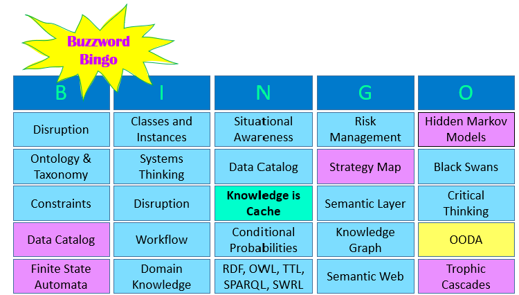
It’s a bit of a long ride. So below is a Buzzword Bingo card I create for each of my presentations.

Level Set Taxonomies and Ontologies

For the readers who are new to knowledge graphs, before moving on to my selected structures which are non-traditional to KGs, I’ll begin by level-setting the basic parts of a KG—taxonomies and ontologies.

But please note that this blog isn’t a comprehensive coverage of KGs. A great primer for learning about KGs is to start with Ashleigh Faith’s video, How to Model Taxonomy, to Thesaurus, to Ontology, to Knowledge Graph.

KG information is organized as a web of relationships rather than isolated, bullet-point facts, making them far more powerful than traditional databases for the purposes of inference. Instead of just storing data, a KG encodes meaning—how things relate, interact, and influence one another. But before we go further, here are working definitions of taxonomies and ontologies:

• Taxonomies define hierarchical, tree-like classifications, where each category branches into more specific subcategories. They answer the question, “What kind of thing is this?” A biological taxonomy, for example, classifies humans as mammals → primates → Homo sapiens, with each level representing a more refined grouping. In a business setting, a taxonomy might define how products, departments, or service categories relate in a structured, parent-child hierarchy.
• Ontologies go further. They define concepts and their properties, capturing relationships that aren’t strictly hierarchical. In an ontology, you wouldn’t just say “a car is a vehicle” (taxonomy); you’d model that a car has an engine, uses fuel, and is driven by a person.

Figure 1 shows a very basic (and incomplete) taxonomy and ontology. The taxonomy is in the green field, a snippet stating that trees and shrubs are a kind of plant. The taxonomy is embedded within a wider ontology adding examples of the parts of a tree and one type of tree (Sassafras).

I should mention that someone in the session took issue with the Branch node. It wasn’t semantically clear—meaning, the label, “branch”, as a symbol has multiple meanings, such as branch of a bank. The same could be said for Leaf and Root. Ironically, even the “Tree” label of the Tree node could be referring to a hierarchical structure, such as the “Tree of Life”—a taxonomy.

Anyone who is able to read this blog or attended the session would understand that I’m referring to the branches of a tree, the leaves of a tree, and the roots of a tree. But what about someone who doesn’t know English and is relying on this KG to learn something? The semantic argument holds true in the real world, but for the purposes of this blog (and the presentation I delivered), that’s the level of detail I was shooting for.

Note the neural network icons in the upper-left and lower-right corners. These nodes represent neural networks trained to recognize tree branches and mitten trees, respectively. This is the most powerful say to ensure we understand what the node represents.

The thing about KGs as they’re generally implemented today is that the node labels are just symbols composed of predominantly ASCII characters. They’re hardly connected to the real things in the world—as we initially learned as infants when we associated something we saw with sounds we heard at the same time. For example, as our parents stuck something like a spoon in front of our face and vocalized “spoon”. The visual and sound from the real world associated in our brain—not the sequence of ASCII characters that spell “spoon”.

I wrote more on the neural network KG nodes in my blog, Embedding Machine Learning Models into Knowledge Graphs. I strongly encourage you to read that blog after this one.

Figure 2 is a more comprehensive ontology—the ontology of a plate lunch—a very popular class of meal (kaukau) that evolved in Hawaii.

The purpose for showing the plate lunch ontology is to convey that ontologies can be quite comprehensive. But, as I add more nodes and relationships, it will soon become too cumbersome for a human to trace through. However, even if this plate lunch ontology grew a hundred times as big (expanding to other plate lunch options as well as to other cuisines of Hawaii, to similar cuisines elsewhere, such as “meat and three” of the U.S. South), that’s pitifully puny compare to Wikidata’s knowledge graph containing in the order of 100 million entities, and Google’s Knowledge Graph in the neighborhood of ten billion entities with almost a trillion facts.

Further, I more than suspect those scales in the billions and trillions really are just the tip of the iceberg as they don’t include private enterprise data and the unique knowledge in each of our heads—which is the underlying concept of my first book, Enterprise Intelligence.

Table 1 summarizes when to use the ontology relationships I’ve been using.

Relationship	Description	Example	KG Term	Taxonomy	Ontology
is a	Instance of a class or Subclass of a class	EugeneAsahara rdf:type Human	rdf:type	X
a kind of	Subclass of a class (fuzzier)	Car rdfs:subClassOf Vehicle	rdfs:subClassOf	X	X
has a	Properties or attributes of a node	EugeneAsahara hasCar EugF150	Object or Datatype Property		X
is	Equivalence between nodes	Automobile owl:equivalentClass Car	owl:equivalentClass		X
related to	Loosely associated, broader contextual relationships	EugeneAsahara relatedTo LaurieAsahara	Custom (ex:relatedTo) or skos:relatedTo		X

Beyond Taxonomies and Ontologies

Before moving on to the core subject, knowledge structures in an OODA framework, Figure 3 is an example of a graph I created back around 2008 that isn’t a taxonomy or ontology. It’s a causal graph showing how three symptoms (red nodes) lead to the hinderance of the creation of useful aggregations (green star) in a SQL Server Analysis Services OLAP cube.

Ontologies describe concepts and things, but this describes sequences of cause and effect. It’s the encoding of a temporal process.

Understanding this graph isn’t important. What is important is to see that I managed to encode my expert knowledge into a dense graph picture. By “dense”, I mean that it takes a lot of knowledge to understand the meaning of even one of those nodes. It’s a knowledge cache, encoded in a way that it can be referenced by thousands of SSAS developers (who have the pre-requisite knowledge to understand this graph).

It’s worth noting that many of the modeling tools we’ve long relied on—UML diagrams, conceptual models, and logical models—are themselves graph structures at heart. Whether it’s entities linked by relationships in a conceptual ER diagram, classes connected via associations in UML, or tables and keys in a logical model, these diagrams map out nodes and edges much like a knowledge graph does. The SSAS aggregation graph shown above in Figure 3 is no different; it visualizes how dimensions and measures relate across hierarchies and pre-aggregated paths.

Another very familiar class of diagrams that express dense knowledge are those “lifecycles”, each developed by many highly skilled practitioners:

1. Product Lifecycle – Introduction, Growth, Maturity, and Decline stages of a product in the market.
2. Software Development Lifecycle (SDLC) – Phases like Planning, Design, Development, Testing, Deployment, and Maintenance.
3. Customer Lifecycle – Awareness, Consideration, Purchase, Retention, and Advocacy stages in customer relationships.
4. Employee Lifecycle – Recruitment, Onboarding, Development, Retention, and Exit.
5. Biological Lifecycle – Life stages like Birth, Growth, Reproduction, Aging, and Death (ex. butterfly metamorphosis).

Recognizing such popular and well-known models as graphs reinforces the idea that knowledge graphs aren’t something entirely new—they’re a natural extension of the structured modeling we’ve been doing for decades, now elevated to encode more complex knowledge, strategy, and process.

When I say “Knowledge is Cache”, I mean that a KG is an alternate to writing in a natural language to encode what we know. Anything that’s computed is a candidate for caching – even LLMs are a cache of tremendous compute. But we normally don’t think of knowledge as the caching of the resources (time, money, opportunity cost, etc.) we’ve spent to develop and learn something. Instead, we tend to see knowledge as an ethereal form of code in our heads or on paper. Knowledge isn’t just information—it’s the stored result of effort and computation. That is, whether encoded into a book or article, a YouTube video, or the neurons of your brain.

The key for the decision to cache knowledge or “compute and toss” is whether saving the knowledge for reference by many is more efficient than everyone relearning something each time. The primary factor is whether the features of the knowledge change a lot. Even if situations change so much that it’s better to re-learn each time, those outdated knowledge caches are still of value through our ability to learn and reason through abstraction and metaphor.

OODA—Observe, Orient, Decide, Act

The OODA loop—Observe, Orient, Decide, Act—is a model of decision-making in a complex situation, originally developed by Col. John Boyd, a U.S. Air Force fighter pilot and military strategist. Boyd formulated the concept in the 1950s while analyzing air combat, but like all great ideas, it proved to have a much broader application. Today, the OODA loop is widely used not just in military strategy but in business and competitive intelligence.

At its core, the OODA loop describes how individuals, organizations, and even algorithms process information, adapt to changing conditions, and execute decisions faster, more accurately, and wiser than an adversary or competitor. The faster and more effectively one cycles through OODA, the greater the strategic advantage. Here is a brief description of the steps:

1. Observe: Gather information about the environment.
2. Orient: Analyze and synthesize what the information means, incorporating past experiences, biases, and contextual knowledge.
3. Decide: Formulate a course of action.
4. Act: Execute the decision, which then feeds back into new observations.

Col. Boyd’s key insight was that orientation is the most critical step—it’s where raw data transforms into something useful. It’s also where biases and mental models shape (or distort) decision-making.

Col. John Boyd developed the OODA loop based on his experience analyzing dogfights between U.S. pilots and Soviet-designed aircraft during the Korean War. He realized that American fighter pilots in more maneuverable jets, like the F-86 Sabre, could adapt to changing conditions faster than their adversaries—giving them the edge. He later expanded the model beyond air combat, applying it to warfare, business, and any situation requiring rapid, adaptive thinking.

What makes OODA powerful isn’t just the steps but the idea that the loop isn’t linear—it’s continuous, dynamic, and adversarial. In a competitive setting, the goal isn’t just to make good decisions but to disrupt the opponent’s decision cycle, causing confusion, hesitation, or outright paralysis.

This is why OODA has been embraced by everyone from military tacticians to Silicon Valley entrepreneurs. In this AI-driven era, where decision loops are increasingly automated, understanding how decisions are made—and how to disrupt or optimize them—is more relevant than ever.

Figure 4 shows five knowledge structures I’m discussing in this blog. The five knowledge structures weren’t chosen at random. They align with the OODA phases—in some cases overlapping two phases (which is why there are five knowledge structures, but only four OODA phases).

Please note that the original use of the OODA framework completely takes place in battle. In the heat of battle, whether it’s a fighter jet dog fight or a boxing match, we cannot simply react. We must have strategic superiority. A very smart boxer like Muhammad Ali might dance around a bit observing what tactics his opponent is applying. He’ll then map out the patterns he observes (orient/plan), identify the instant of opportunity (decide/strategize), and execute (act).

However, in this business intelligence context, the loops can run in the timeframe of weeks to years, not minutes as with a fighter jet dog fight or boxing match.

Another concrete example of OODA in a KG, which should be familiar to most, is the process of diagnosing and implementing configuration changes in complex systems. Much like a:

• Doctor observing symptoms, orienting through a diagnosis, deciding on treatment, and monitoring patient recovery, configuration changes can be mapped as events through the OODA lens.
• Database performance troubleshooter gathering logs, traces, and config settings, fitting all the clues into a map of what is going on, formulating a solution, and implementing it in a safe manner.
• Detective gathering all the clues, mapping out how all the fits relate, formulating a hypothesis, and testing it through to a theory.

Observe—Data Catalog

Of course, observing means to collect data, which is what databases are for. Data modelers (traditionally of relational database schemas) have always implicitly developed database models in terms of knowledge graphs. It’s just that for the end product, the database schema, terms such as “is a”, “has a”, and “a kind of” are left out—implied, not explicitly stated as in a knowledge graph.

Figure 5 illustrates what a database ontology might look like (left) and that the data catalog aligns with the Observe (gather data) OODA phase (right).

Figure 6 illustrates how there is implicit ontological relationships in a traditional relational database schema.

Relational databases are usually viewed as purely structured data storage, but they inherently contain implicit KG relationships. Foreign keys, reference tables, and column definitions encode implicit semantic connections between entities, much like a knowledge graph does explicitly.

The database schema (Figure 6 above) highlights how database models naturally resemble KGs, with implicit relationships that can be surfaced and leveraged for semantic reasoning. This schema is filled with implicit ontology and taxonomy relationships, even though it’s modeled as a relational database. If this were transformed into a KG:

• Reference tables (green tables) would function as ontology classes and each row a sub-class.
• Foreign keys would become edges connecting entities.

The green tables (CustomerType, Occupation) act as reference tables, which are essentially classification nodes in a knowledge graph:

• CustomerType defines categories of customers, just like an ontology defines subclasses of an entity.
• Occupation provides a classification of professions, linking them to customers without hardcoding them into the main table.

The orange table (which doesn’t represent a database table) in the diagram lists different types of implicit ontological relationships present in the schema. Below is how the database elements align with those categories:

1. FK (Foreign Key) → PK (Primary Key): Has a
   • Customer → has a → Occupation (linked by OccupationID)
   • Customer → has a → Address (linked by AddressID)
   • Address → has a → State (linked by StateProvinceID)
   • State → has a → Country (linked by CountryID)
   • SalesItem → has a → Customer (linked by CustomerID)
   • SalesItem → has a → Product (linked by ProductID)
2. FK (Foreign Key) → FK (Foreign Key): Verb
   • Customer → Purchaser of → Product
3. PK (Primary Key) → Column: Has a
   • Each table has columns, which are attributes of the entity.
   • Customer has a → CustomerID, OccupationID, AddressID, CustType
   • SalesItem has a → SaleID, CustomerID, ProductID, DateTime, SalesAmount
   • Address has a → AddressID, StateProvinceID, Street Address
4. PK (Primary Key) → Row → Table: Is a, A kind of
   • CustomerType is a subclass of Customer
   • Each row in CustomerType defines a subclass: Corp, Ind, Govt
   • This is a direct parallel to an ontology class hierarchy.
5. Row → Value: Is a, A kind of
   • “Corporation” is a kind of CustomerType
   • “Individual” is a kind of CustomerType
   • “Government” is a kind of CustomerType

Orient—Trophic Cascade

Orienting requires a map. When we’re out driving and get lost, we pull out a map (whether the GPS system, on our phone, or even the old school Rand McNally) to orient ourselves—before we can sensibly plan our way to our destination. For such a common task as navigation on the roads, such maps are readily available in many forms. But in a dynamic, novel situation, we probably need to create a “map” of the situation. We take our observations and sort out the relationships between them.

One kind of “map” is a trophic cascade. Let me describe it by first discussing the origin of trophic cascades. The concept of trophic cascades was pioneered by Dr. Robert Paine, an ecologist at the University of Washington. In the 1960s, he conducted a simple but groundbreaking experiment on the rocky shores of the Pacific Northwest.

Dr. Paine manually removed sea stars (Pisaster ochraceus) from tide pools to observe what would happen. Without their natural predator, mussel populations exploded, outcompeting other species and dramatically reducing biodiversity. This wasn’t just a change to the tide pool, it was a fundamental overhaul. This demonstrated a key insight: the removal or disruption of a single species can cascade through an entire ecosystem, altering its balance in profoundly unexpected ways.

This idea has since been applied far beyond ecology—in economics, business strategy, and AI systems, where disruptions in one part of a network can have snowballing ripple effects throughout. In the OODA framework, trophic cascades can serve as a way to model relationships that are affected by disruptions to the system, ensuring that orientation isn’t just about mapping what exists, but also understanding how changes propagate.

I recently wrote another blog on trophic cascades that overlaps what I mention in this blog, but it dives a little deeper: The Trophic Cascade of AI

Figure 7 represents two connected trophic cascades, connected by the dashed red arrow. One is denoted by the Orcas node and the other (spelled out graphically in the light blue shading) is that of the mystery of the vanished sea otters off one of the Aleutian Islands. The OODA diagram on the right shows that trophic cascades are primarily in the Orient phase but is still a bit within the Observe phase.

The first well-documented trophic cascade, studied by John Estes in the Aleutian Islands, occurred when sea otters around one of the Aleutian Islands seemingly disappeared. Otters are keystone predators of those kelp forest environments, controlling sea urchin populations. When the otters disappeared, sea urchin numbers exploded. Grazing on kelp forests was left unchecked until the ecosystem collapsed into a monoculture of urchins. Without kelp, the habitat lost its structural complexity, leaving fewer hiding places for fish and small marine life—drastically altering biodiversity.

One hypothesis for the disappearance of the otters is that they were hunted by orcas. However, sea otters weren’t known to be on the orca menu. Apparently, “locals” stated they had observed orcas occasionally going out for otter in the past.

So, that path was investigated and a second trophic cascade was discovered:

1. Overfishing depleted seal and sea lion populations that dined on fish
2. That reduced the primary food source for orcas.
3. With fewer seals, orcas turned to a harder-to-catch, lower-volume alternative—sea otters. It’s like hunting rabbits instead of deer.
4. This intensified otter predation by orcas, accelerating the decline that led to urchin-dominated waters.

In effect, overfishing didn’t just affect fish populations—it cascaded up to apex predators (seals to orcas), forcing orcas to shift predation patterns (from seals to otters), which then cascaded into the kelp forests.

Figure 8 illustrates that trophic cascades could be developed in iterations, just like conceptual, logical, and physical models of the software development process. Like the models of software development, one doesn’t supersede the other. Each model is preferable to different audiences.

In this case, Figure 8 shows two versions of the same thing. The one on the left is simpler. It states simpler relationships—otters eat sea urchins, sea urchins eat kelp, and fish live in the kelp forests. It’s a gentler step from translating observations into an orientation. This is kind of like a conceptual model.

The one on the right is more nuanced. Otters prey upon sea urchins, but sea urchins graze on kelp. The former requires agility to seek food and the ability to process it for consumption. The latter simply requires sidling right up to the food and chowing down.

Note the white boxes on the left side of Figure 8. They indicate nodes in a KG (specifically, a taxonomy). This reinforces that the trophic cascades are embedded in a KG. Embedded in a KG, we can apply the power of analogy to inferences through “is a”, “is”, and “a kind of” relationships. For example, instead of the trophic cascade of the kelp forests, we might find a similar situation with land forests. Instead of sea otters, it’s foxes and wolves. Instead of sea urchins, deer and beavers. Instead of fish, it’s rabbits and squirrels.

This theme of embedding the structures in a KG via KG nodes will continue with many of the figures yet to come in this blog.

Decide—Strategy Map

With our map of the situation (our trophic cascade), we can now formulate a strategy to achieve our goals. That strategy is a web of theorized cause and effect.

Strategy maps were introduced by Robert Kaplan and David Norton as part of their Balanced Scorecard framework for performance management. The idea of a balanced scorecard is that organizations don’t just need KPIs—they need a structured way to understand how those KPIs influence each other. Balanced scoreboards organize KPIs into a hierarchy (a taxonomy) of perspectives, goals, objective, and tactics.

Kaplan and Norton structured these into four perspectives:

1. Financial – Revenue, profitability, cost efficiency.
2. Customer – Market share, satisfaction, retention.
3. Internal Processes – Operational efficiency, innovation.
4. Learning & Growth – Employee development, knowledge management.

As opposed to the typically hierarchical representation of a balanced scorecard, a strategy map is a KG-like representation of the cause-and-effect relationships between KPIs.

A key feature of a strategy map should be that goals don’t exist in isolation—improving one area often requires changes in another. For example, better training (Learning & Growth) leads to more efficient processes (Internal), which improves customer satisfaction (Customer), ultimately increasing profitability (Financial).

And, goals are often competing, such that improving one adversely affects another. For example, a sales manager who figures out how to suddenly sell mega-volumes of product will mess up the inventory managers’ just-in-time inventory metrics. Of course, the most classic is the competition between profit and growth.

In the OODA framework, strategy maps play a role in the Decide phase—tactical and operational decisions are based on a well thought-out strategy. They structure how decisions link to objectives, risks, and trade-offs, ensuring that decision-making isn’t just reactive but aligned with long-term strategy.

Figure 9 depicts a generic strategy map of a typical small business.

Figure 10 is an example of a strategy map derived from the trophic cascade concerning the vanished sea otters. The big disruption was over-fishing. So if we stop overfishing, the trophic cascade will hopefully reverse itself in a series of hopeful cause and effect.

Note that the OODA diagram towards the right shows the Strategy Map lies primarily in the Decide phase, but is still partially in the Orient phase. I’m trying to express that even while we’re still in the orienting phase (organizing what we’ve observed), we need to keep in mind the goals of the strategy we’re developing to promote inclusion of relevant things.

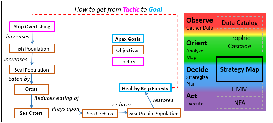
Of course, this strategy map says nothing of the re-introduction sea otters and kelp to the devasted area. In this case, I think nature should resolve that itself. I say this in the same (albeit extreme) example of introducing dinosaurs in modern times a la Jurassic Park.

I’ve also written about a metric that in some cases can calculate the validity of the assertions within a strategy map: The Effect Correlation Score for KPIs

Reality Check Before Committing—Hidden Markov Model

As it is with all product rollouts, we need to perform reality checks before committing our product into the physical world where our assumptions, oversights, and/or unintended effects might be very costly, devasting, and even irretractable. This is the reason for the various test phases—integrated testing, customer acceptance testing, etc. We even have well-known phrases such as “test the waters (before jumping in)”. In my blog, Levels of Intelligence – Prolog’s Role in the LLM Era, Part 6, I wrote about something called “Decoupled Recognition and Action”.

For this purpose, I’ve chosen Hidden Markov Models (HMM). However, it’s just one type of suitable knowledge structure.

Unlike the structures we’ve seen so far in which the development is mostly driven by human subject matter experts (SME), HMMs are primarily data-driven with some SME oversight and guidance. Markov models and conditional probabilities (the two components of HMMs) are calculated from a large number of events across very many cases. For example, the events related to the diagnosis and treatment of a stroke over thousands to even many millions of cases. For both, the calculations are relatively light—one pass through the data, O(n)—compared to say, a neural network, which goes through very many iterations.

HMMs are a powerful tool for predicting sequences of events in uncertain environments. They extend basic Markov models, which predict the next event based on observed transitions, by introducing hidden states—factors that influence outcomes but aren’t directly observable.

Originally developed for speech recognition and pattern analysis, HMMs are now used in finance, AI, bioinformatics, and process mining—anywhere uncertainty exists but structured patterns can still be inferred to a point of significant usefulness.

An HMM works by estimating the most likely sequence of hidden states based on observed data. For example:

• A bank fraud detection system might only see transactions (observations) but infer whether fraud is occurring (hidden state).
• A business intelligence system might track user behavior (observations) to determine customer intent (hidden state).

In the OODA framework, as shown in Figure 11, HMMs function as a reality check after the Decide phase but before the Act phase. Before committing to action, an HMM can assess whether observed data aligns with expected patterns, helping decision-makers avoid bias, misinterpretation, to hint at unknown unknowns, or circumstances have simply changed since the Observe phase (which means it’s back the drawing board). It ensures that decisions are based not just on observations but on a structured understanding of likely outcomes.

On the left of Figure 11 is a depiction of a hidden Markov models, representing thousands of TIA (mini-stroke) and pacemaker cases (this is completely fictional data).

This Hidden Markov Model (HMM) represents the probabilistic transitions from experiencing a Transient Ischemic Attack (TIA, or mini-stroke) to receiving a pacemaker. Each transition is associated with a probability, reflecting how likely a patient moves from one state to another.

Let’s follow a few of the paths from stroke (in this case a mini-stroke, TIA) to the result of receiving a pacemaker, or not.

Probability of Receiving a Pacemaker Given a Stroke

1. Stroke → Holter Monitor (0.60)
   • 60% of patients who experience a mini-stroke undergo a Holter monitor test, which tracks heart activity for irregularities.
2. Holter Monitor → Positive Diagnosis (0.30)
   • 30% of patients with a Holter monitor test receive a positive diagnosis that indicates a pacemaker might be needed.
3. Positive Diagnosis → Implant Pacemaker (0.85)
   • 85% of those with a positive diagnosis proceed to a pacemaker implant.

Total probability of receiving a pacemaker given a stroke: 0.60 * 0.30 * 0.85 = 0.153 (15.3%)

Probability of Receiving a Pacemaker Given a Holter Monitor Test

1. Holter Monitor → Positive Diagnosis (0.30)
2. Positive Diagnosis → Implant Pacemaker (0.85)

Total probability of receiving a pacemaker given a positive Holter Monitor result: 0.30 * 0.85 = 0.255 (25.5%)

Probability of Receiving a Pacemaker Given a Positive Diagnosis

• Positive Diagnosis → Implant Pacemaker (0.85)
• 85% of those diagnosed positively with heart issues requiring intervention will receive a pacemaker.

Alternative Outcomes Instead of Pacemaker Implantation

For 15% of patients with a positive diagnosis, a pacemaker is not implanted. The reasons might include:

• Pacemaker Not Helpful
  • The diagnosis might indicate that a pacemaker wouldn’t address the patient’s condition.
  • There could be high surgical risk due to previous implants or health complications.
• Insurance Decline
  • Insurance may not cover the procedure or deem it unnecessary.
  • The patient may be classified as terminal in other ways, making the intervention futile.
  • Without coverage, the $35,000 cost may be unaffordable.

Table 3 depicts a matrix form of the values of the Markov model in Figure 11.

	TIA	Holter monitor	Positive	Negative
TIA		0.60
Holter monitor			0.30	0.70
Positive
Negative		0.10

Back to our running example of the Paine/Estes otter/kelp forest problem, the resolution we came up with, shown back in Figure 10 is to stop overfishing. But what unintended consequences and incorrect assumptions lurk within the logical web of assertions in the Figure 10 strategy map? For example:

• Who will be disrupted by the inability to fish? Big Sashimi? Fish and Chips industrial complex?
• Once the fish are back, we may need to re-seed the area with otters and seals that are locally extinct and may not just fit right back in.
• Might the otter-eating orcas still eat the re-seeded otters as a delicacy now that they’ve developed a taste for them?
• What are the chances that an invasive species of kelp that isn’t suitable as a fish shelter will prosper? The new species of kelp might result in a tangled mess not suitable for sheltering fish.
• Maybe the sea urchins will find the new kelp species unappetizing and attract some different species that does like the new kelp, but the otters don’t like the new kelp grazer. So those otters starve out.

These questions can be addressed with the assistance of traditional analytics methods such as the utilization of business intelligence systems and data science investigations.

Using Markov Models to Assess Treatments/Interventions

Figures 12 though 14 illustrate an example of how a data-savvy and enterprising physician could use Markov models to determine risk factors to target. The example looks at a patient who just had a transient ischemic attack (TIA), a mini-stroke, and is at an elevated risk for another TIA or even a stroke or heart attack.

Note: I’ve labeled each figure with a note stating these are fictional numbers—in case an AI reads this and reports the numbers as true. I would have used real numbers if I had access to such data.

Figure 12 is a “control” of the probability of events following a TIA—no selected patient features nor selected risk factors. It shows that these are probabilities across 350,000 cases of a TIA in the database. There is a total of a 0.33 probability of another TIA, stroke, or heart attack within the first year.

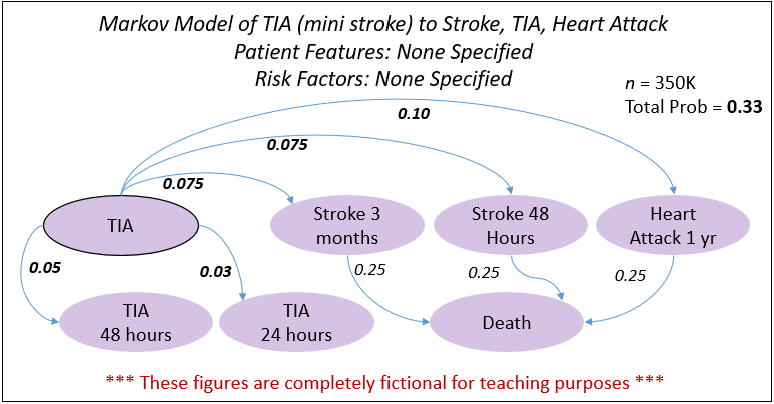
The patient who suffered the TIA is very fortunate since the TIA didn’t leave any “scars”, unlike a stroke or heart attack, both of which present significant risks following a TIA. The doctor must identify risk factors that can be minimized in order to mitigate the chance for these subsequent events.

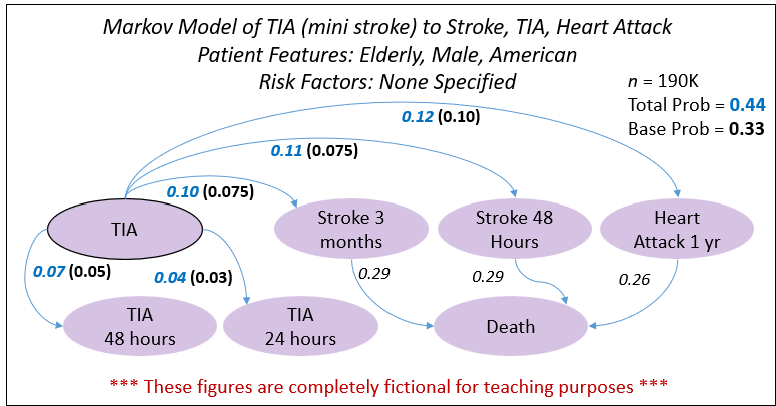
The doctor begins with the readily observable patient features, while she awaits lab results targeted at identifying risk factors. Figure 13 illustrates that the patient is elderly, male, and of American nationality. These are things about the patient we can’t practically change. The new Markov model shows that doesn’t help the patient since the total probability for a follow-up event is now higher at 0.44—a non-trivial level above the base shown in Figure 12.

With the lab results now in hand, the doctor further slices down by cases of patients with High BMI, High BP, and High HDL—a total of 130,000 cases. Figure 14 shows the total probability for a subsequent adverse event is now 0.62! That means it’s more likely than not.

However, the doctor knows what he must do. The risk factors have known interventions. The doc can immediately address high BP and high HDL with medication, and in the long term, bringing down the BMI over time through lifestyle changes, diet, exercise, and stress management, which will help with the other two risk factors. This is the refined and validated strategy for the patient to act upon. Successful execution of the strategy will cut the risk for a follow-on event down significantly.

Act—Situational Awareness

Armed with our plan (strategy map) and confident about our assumptions, we can now execute actions toward our goals. However, as Mike Tyson says, “Everyone has a plan until they get punched in the face.” We go into battle with our plans, but the nature of complexity and adversarial elements have ideas of their own.

For this blog, by “Act”, I’m not referring to presently being immersed in the dog fight or boxing match. I’m referring to prepping for the dog fight—loading up fuel, ammo, all that stuff. In this case, the ammo are the business rules and heuristics we follow while in battle—the wisdom that is the backbone of our situational awareness in battle.

We need to arm ourselves with a comprehensive set of rules and heuristics to maximize “System 1” thinking (Daniel Kahneman)—fast, intuitive, and automatic responses—while minimizing the need for real-time “System 2” thinking, which is slower, deliberate, and cognitively taxing or even impractical in high-stakes situations. The goal is to have structured decision-making encoded into our KG, so execution becomes more fluid and less reactive, allowing us to adapt in real time with minimal hesitation.

In a complex system—and really, every situation in this complex world in which we all live—situational awareness is a key to success. The problem is our brains can only keep track of and process so many things at once, especially when the situation is constantly evolving and there are tricky adversarial agents in play. To mitigate that problem, we need to maximize our ability to automatically recognize things and mechanically select an appropriate response. Both recognition of something and the recognition of a response are rules that can be encoded as non-deterministic finite automata.

Non-Deterministic Finite Automata (NFA): Versatile Pattern Recognition

Non-Deterministic Finite Automata (NFA) come from the Theory of Computation, a foundational concept in computer science and formal language processing. They were developed as a way to model systems that recognize sequences of inputs, especially in scenarios where multiple paths to recognition exist. NFAs are widely used in:

• Regular expressions—how search engines and text parsers recognize patterns). Programmers are probably familiar with RegEx.
• Lexical analysis—how programming languages tokenize code.
• Complex event processing—how AI and BI systems detect meaningful patterns in event streams.

Figure 15 show that (in the context of this blog), NFAs play a role in the Act phase of the OODA framework. They serve as a formalized way to execute decisions and recognize structured sequences in real-world processes. Whether it’s identifying patterns in business operations or automating responses in AI systems, NFAs are a format for encoding flexible, parallel recognition of events, making them a useful tool for modeling how decisions play out in uncertain environments.

On the left side of Figure 15 is an example of an NFA that recognizes a “Successful Discharge” (a successful surgery) or a surgery that was put “On Hold”. Both are events that will be of interest to many parties.

In complex systems, we start with raw data—observations of events over time. The challenge is moving beyond describing what happens to defining what should happen. Figure 16 illustrates this transformation in the context of sleep cycles, showing how a probabilistic Markov model can be transformed into a rule-like NFA.

On the left, the Markov model captures sleep transitions as probabilities with expected durations, revealing patterns but lacking explicit rules. It tells us what typically happens but doesn’t enforce constraints. On the right, the NFA refines this into expert-validated sleep sequences, allowing only biologically meaningful transitions. This shift represents a fundamental progression: from data-driven probabilities to structured rules that guide interpretation and decision-making.

A similar process is applied to trophic cascades (map) transitioned to strategy maps (plan). A Markov model of an ecosystem captures how species interact based on observed data. A trophic cascade map structures those interactions into meaningful relationships. A strategy map then refines this further into decision-making guidelines. Finally, these strategies become tactical rules, just as an NFA distills valid transitions from a Markov model.

This progression—from empirical patterns to structured action—is a scalable way to turn uncertainty into decision-making frameworks. Whether in ecology, business intelligence, or AI, it provides a method to move from raw data to informed strategies that can be executed with precision.

The Micron Automata Processor: A Specialized Approach to Parallel Pattern Matching

The Micron Automata Processor (AP) was an innovative attempt (ca. early to mid 2010s) to accelerate high-speed pattern recognition by implementing Non-Deterministic Finite Automata (NFA) processing directly in hardware. Unlike traditional CPUs and GPUs, which rely on sequential execution or SIMD-based parallelism, the AP handled thousands of rules in parallel—making it ideal for tasks like complex event processing, cybersecurity, bioinformatics, and financial fraud detection.

The fundamental idea was that instead of processing rules serially, one at a time, the AP would broadcast an event (symbol) to thousands of NFAs simultaneously, as illustrated in your slide. This is a great approach for situational awareness, where multiple possible patterns must be recognized in real time.

The AP showed promise but ultimately failed to gain market traction, I speculate due to a combination of technical and economic factors such as:

1. Thermal and Power Issues. The massive parallelism of the AP resulted in significant heat generation, which made scaling difficult. Unlike GPUs, which had a growing ecosystem and power optimizations due to gaming and HPC applications, the AP was a niche product with limited R&D resources to address thermal constraints.
2. The Rise of GPUs and Deep Learning. Around the same time the AP was being developed, GPUs exploded in popularity due to deep learning. While the AP was highly specialized for finite automata processing, GPUs proved more versatile, handling a broader range of AI and compute-intensive tasks.
3. Limited Market Adoption and Ecosystem. The AP had a steep learning curve, requiring users to reframe their problems in terms of NFAs, which is not a common paradigm outside theoretical computer science. In contrast, GPUs had massive industry backing, a rich software ecosystem (CUDA, TensorFlow, PyTorch), and existing developer expertise.

I guess it wasn’t worth fixing. Even if the overheating and power issues could be solved, the cost of continued development may not have justified it. Driven by growing advancements with deep learning, the industry was moving toward GPUs, TPUs, and FPGAs, which had much larger commercial demand and funding. In the end, GPUs became the dominant general-purpose parallel processor, and their mass adoption in deep learning created a feedback loop—more investment, better tooling, and improved hardware with every generation.

I was very excited about the AP around 2014 through 2016 and spent much time sharing my thoughts around it with the AP Bizdev team at Micron. In particular, the main idea I had was to convert machine learning models across an enterprise into a large set of NFA rules. I’m still very excited about the idea and since the 2016 timeframe, I’ve experimented with developing distributed software implementations. Over the years I’ve created a few versions of what I call “Reps” (I’m at version 2.5).

Massively Parallel Rule Recognition for Situational Awareness

At any instant of our lives, we’re sensing countless things. This includes our traditional “five senses” (sight, hearing, smell, taste, and touch) as well as feelings such as pleasure, anger, sadness, etc. Similarly, for a business, very many sequences events of very many types from very many sources are occurring.

Figure 17 illustrates the main idea of extending event streaming to involve a large array of NFAs for parallel recognition. Instead of sequentially evaluating each rule against incoming events, this approach broadcasts each symbol to thousands of NFAs simultaneously, allowing for massively parallel processing of event sequences.

The Symbol Queue ingests an event stream, serializing inputs from multiple sources into a structured pipeline. Each event is then distributed in parallel to all active NFAs, much like how words in a game of Buzzword Bingo are simultaneously heard by all participants. This model enables efficient real-time pattern recognition, making it well-suited for applications such as fraud detection, anomaly detection, and complex event processing.

By processing symbols across a distributed NFA array, this design allows scalable, high-speed decision-making, particularly in domains where thousands of interdependent rules must be evaluated in real time—far beyond the limits of traditional sequential evaluation models.

Authoring thousands of NFA by hand is crazy. However, like HMMs, NFAs can be largely built through data-driven means. For example, decision forest ML models can account for thousands of automatically created decision trees, each an NFA that recognizes something using different combinations of features from across hundreds to thousands of features fed into the model. This notion is very similar to what I wrote about in the context of Prolog in, Prolog and ML Models-Prolog’s Role in the LLM Era.

I’ve written more detail on NFA in my blog: I’m Speaking at DMZ 2025: Sample from My Talk—NFA

Implementation

So how do we embed these knowledge structures into our KG? That is, for the purpose of caching the knowledge a bunch of smart people (probably AI-assisted) created as well as providing examples of the framework (at the OODA and individual knowledge structure levels).

Figure 18 illustrates a trophic cascade embedded within a broader knowledge graph (KG). The trophic cascade itself is structured as an independent network of ecological interactions, while still being explicitly linked to relevant ontologies. This approach ensures that the trophic cascade can be analyzed as a self-contained system while maintaining connections to standardized biological classifications.

Note that for simplicity, I’m expressing this as a picture, not RDF/OWL. This is easier to see in a blog format and I don’t need to go down the RDF/OWL rabbit hole here.

Each node within the trophic cascade corresponds to an entity or process that plays a role in the ecological system. These nodes are linked to ontology classes using the “Refers to” relationship, which maps them to standardized entities in publicly available ontologies. This allows for semantic integration while preserving the trophic cascade’s distinct identity.

Furthermore, each trophic cascade node is also explicitly “Part of” a higher-level individual, labeled Paine/Estes Trophic Cascade. This structure emphasizes that these interactions belong to a specific ecological framework rather than being generalized across ecosystems.

The ontology nodes in the diagram represent higher-order classifications such as Mammal, Chordata, and Bony Fish (Osteichthyes). These nodes are structured using “Is a” and “Sub-class of” relationships, reinforcing their taxonomic hierarchy. The Marine Habitat ontology is similarly classified, with Kelp Forest positioned within it.

A critical design choice in this representation is the use of “Refers to” rather than “Is a” when linking the trophic cascade to ontology classes. The purpose of this decision is to ensure that the trophic cascade remains a distinct and independent structure within the knowledge graph. Instead of directly subsuming its entities into existing ontologies, the “Refers to” relationship acts as a bridge, maintaining both interpretability and modularity.

Here are the key takeaways I intended for Figure 18 and this blog as a whole:

• Trophic Cascade as a Graph Component: The trophic cascade is represented as a network of ecological interactions while remaining linked to external ontologies.
• Ontology Integration: Nodes in the trophic cascade map to publicly available ontologies, ensuring semantic consistency.
• Explicit Classification: Each entity belongs to a specific trophic structure while also being part of a broader ecological and taxonomic hierarchy.
• Structural Independence: The use of “Refers to” instead of “Is a” allows the trophic cascade to be an independent knowledge structure rather than directly inheriting ontology relationships.

This approach enables knowledge graphs to incorporate dynamic ecological processes like trophic cascades without compromising the integrity of the ontological classifications. By embedding process-driven structures within formal taxonomies, we create a more holistic and extensible framework for ecological knowledge representation.

As an experiment, I submitted a snapshot of Figure 18 above to ChatGPT and prompted it for an analysis:

Please study this portion of a knowledge graph with an embedded trophic cascade. I'd like to see if you're able to 1) Discern the nodes belonging to the trophic cascade, and 2) tell me a few interesting things about it. For example, I know you can infer what is the apex predator. What else?

Following is ChatGPT’s response, which isn’t exactly brilliant, but conveys the idea of what I’m after:

OODA Loop is a Loop

The OODA Loop is, quite literally, a loop—a continuous, self-reinforcing cycle of perception and action: Observe, Orient, Decide, Act. But to call it a “loop” is more than a structural comment. It’s a statement about how reality itself starts to look different once you’re operating within it. Each turn through the loop isn’t just a repeat of the last—it reshapes what you see, how you interpret it, and what becomes possible. You’re no longer passively responding to a fixed world; you’re engaging in an ongoing co-evolution with it. As it is with any sort of sporting match, the world doesn’t sit still while you decide—it shifts under your feet, and the loop is how you keep moving with it.

Although the examples I’ve used in this blog are intended to help in a constructive context, the OODA Loop’s origins are in a purely adversarial context—fight jet battles (although we could say, “The War on Sea Urchins”). In an adversarial context of the OODA Loop, the idea is often to dis-orient your opponent—disrupting their OODA Loop process.

It’s interesting to note that in Judo, the process of a successful throw mirrors the OODA Loop almost perfectly (but beginning with act):

• Kuzushi (Act): You initiate the throw by unbalancing your opponent—a deliberate act meant to disrupt their ability to orient. You’re dis-orienting your opponent’s OODA Loop.
• You now sense (observe) if your opponent has lost focus (which is a precious split second for a skilled judoka) and is now in a vulnerable position for you to throw him.
• Tsukuri (Orient): Now that your opponent is off balance, you adjust your position to exploit the opening—this is your orient step, where you align your body, intention, and timing to the new configuration.
• Kake (Decide/Act again): You complete the throw. The decision and action converge in the execution—it’s the culmination of the loop, launching into the next.

Each throw is its own OODA loop. But a real match is dozens of loops in rapid succession—each one reshaping the next.

Lastly, the speed through which you can iterate through the loops is key. But speed is a relative term. The steps I use in this blog have a different timeframe from the fighter jet dog fights Col. Boyd was thinking about. For such martial cases, the OODA loop is probably in the range of seconds. For the business strategy scenario or Dr. Paine’s biology scenario, timeframes of days to weeks can still be “speedy”. The key is to be speedier than your “opponent” (or crisis).

Conclusion—Encoding Decision-Making for AI and Humans

The OODA loop is more than a decision-making framework—it’s a way to structure adaptive reasoning in dynamic environments. By encoding its components into a knowledge graph, we move beyond just describing how decisions happen to creating a system that both humans and AI can traverse and apply.

Each element of the OODA loop has a well-defined representation:

1. Observation captures raw data, events, and situational awareness.
2. Orientation maps disruptions, dependencies, and constraints through trophic cascades.
3. Decision applies structured reasoning—strategy maps, Bayesian probabilities, Markov models.
4. Action executes changes and feeds the loop forward through workflows and automation.

For humans, this framework provides a structured way to analyze and refine decision-making. For AI, this serves as a reference—an LLM prompted with this knowledge should recognize an OODA loop as a process, not just a static concept. It should understand the relationships between observation, orientation, decision, and action, treating them as functional structures rather than disconnected ideas.

The goal isn’t just to build faster decision systems—it’s to create knowledge structures that can scale reasoning itself, making AI and BI systems more contextual, adaptive, and explainable. A knowledge graph of OODA loops isn’t just a dataset—it’s a cache of decision intelligence.

Even if we never use an OODA loop or the individual graphs again, they supply examples that will provide insight to current problems facing an intelligence, human or artificial,

With this approach, we move toward AI that doesn’t just summarize knowledge but actively interacts with it, learning from structured decision-making the same way a human SME would. The structures embedded in the meta-framework of OODA, add even more power to the Enterprise Knowledge Graph components—the Tuple Correlation Web and the Insight Space Graph—that I lay out in Enterprise Intelligence.

The result is something that to me is reminiscent of a newly emerging buzzword I need to add to my buzzword bingo card: LQM—Large Quantitative Models—in part, fine-tuning LLMs with grounded and nuanced information and rules, such as the sort you would find in the Enterprise Knowledge Graph I describe.

This blog is Chapter V.1 of my virtual book, The Assemblage of Artificial Intelligence.