The Ghost of OLAP Aggregations – Part 1 – Pre-Aggregation

If your entry into the business intelligence (BI) game began after around 2010, it could be difficult to appreciate the value of OLAP cubes (referring mostly to SQL Server Analysis Services MD, ca. 1998-2010), those aggregations, and that MDX query language. In fact, you may have a negative impression of those relics, those “cubes”, based on the experience of those who began their BI implementation efforts well before 2010. And with good reason. Back in those bad ol’ days:

• OLAP cubes required big and expensive servers that were very difficult to implement and maintain.
• It was extremely difficult to map entities across domain software across the enterprise—before master data management and AI (mostly in the form of natural language processing) matured enough to be helpful.
• OLAP cubes worked nothing like the relational databases (like SQL Server and Oracle) database folks were used to. And they came with a whole other query language, MDX. Remember though, OLAP cubes were really the OG NoSQL technology.
• The “analytics” cultures at enterprises were very much a nice-to-have, not mission-critical. The MBAs plodded along with Excel spreadsheets scattered across all their desktops.

After 2010, during the buildup days of in-memory processing, MPP data warehouses (massively parallel processing, ex. Snowflake, SQL Server PDW, Netezza), Big Data, Spark (Databricks), and the Cloud, the hardware infrastructure was sufficient to support the vast majority of analytical use cases without cubes, even at scale. So the role of OLAP cubes, the BI staple from the mid 1990s through 2010, took a back seat. Similarly, AI has taken those technologies out of the spotlight since late 2022. But none of those things went away.

I can imagine Mr. Burns from the Simpsons yelling, “Smithers! Fetch me my OLAP cube!”

So why should you read this? Because when the volume of data exceeds the ability of the current data platforms to process effectively, optimization should be the first option. OLAP cubes were the optimization created for the problem of the inability to effectively analyze OLTP data back in the 1990s. They became an option to avoid buying ever larger systems. Back then, the SMP servers were scale-up, where its cost scaled-up much faster than the server capacity—the phrase was “throw more iron at it”. The other option was to continue depending on human MBAs if you had them, hoping for the day that something magic that we’d later call “The Cloud” came about … or do nothing.

But this blog isn’t about the justification for OLAP cubes in this day of AI. One of my books, Enterprise Intelligence, is all about that. And I wrote a few blogs on that justification:

• The Role of OLAP Cube Concurrency Performance in the AI Era
• The Effect of Recent AI Developments on BI Data Volume
• The Need for OLAP in the Cloud

This blog is about the seemingly dull subject of optimization of a BI platform, specifically pre-aggregations of OLAP cubes. It’s dull to IT people because optimization requires even more discipline, added effort, possibly yet another product in the stack, and the ongoing cost of maintaining it. It’s dull to the end users because they just want things to work. It’s dull to manufacturers because it impedes further sales of the products we’re optimizing.

Optimization is the other side of the hill after innovation—long periods of evolution following a disrupting revolution. This probably sounds odd at this time of major disruption by AI. But the optimization I’m talking about is the optimization of a solid BI foundation. It’s the foundation that has gathered data from across the enterprise and laid it out into a cleansed, high-quality, secured, user-friendly, and highly-performant bedrock on top of which we can innovate through analysis.

Products such as SQL Server Analysis Services (SSAS), Cognos, and today, Kyvos, are built around this interaction model. Users “drag and drop” dimensions into rows and columns, and measures are aggregated automatically—behind the scenes, this is a slice and dice query.

This pattern is heavily used by BI consumers, traditionally anyone with “analyst” or “manager” in their title, working in tools like Tableau, Power BI, Looker, or Qlik. These users rely on slice and dice operations to explore data across different dimensions, spot trends, identify outliers, and generate reports—all without writing SQL themselves.

This blog, “The Ghost of OLAP Aggregations – Part 1” is actually “Part 3” of a series on OLAP cube fundamentals. That is, after all the Big Data, Data Science, and Cloud era and especially in this crazy AI-disrupted time. It is intended for the current generation of analytics engineers who began after 2010 and didn’t get to know OLAP:

1. The Ghost of MDX – Overview of subcubes and aggregations. Requisites for MDX.
2. An MDX Primer – Later, you might want to get the gist of MDX. It encapsulates the functions of analytical querying.
3. The Ghost of OLAP Aggregations – Part 1 – Pre-Aggregations
4. The Ghost of OLAP Aggregations – Part 2 – Aggregation Manager

This blog is a moderately technical description of aggregations and how they affect query performance and concurrency. Aggregations are about the preservation of compute—Process once, read many times. It’s about mitigation of redundant compute across a massive volume of data. Preservation of compute can be used towards:

• Faster query response time.
• Higher concurrency. Enable more concurrent queries as the population of BI consumers increases from a relative handful of managers, analysts, and data scientists to:
  • Tens of thousands of knowledge workers throughout an enterprise.
  • What could quickly become million to billions of AI agents.
  • What could become trillions of IoT devices.
• Conservation of resources—compute costs which benefits the enterprise, and conservation of energy which benefits everyone (and is a primary topic today because of the ridiculously high compute requirements for AI).

In “The Ghost of OLAP Aggregations – Part 2”, I’ll describe the other part of an OLAP cube product. It’s not just about aggregations, but more importantly, the management of the aggregations. My blog, All Roads Lead to OLAP Cubes… Eventually, gives you a good idea of that value.

It’s important to understand that the examples that follow are SQL queries on a SQL Server database (the famous AdventureWorksDW). There are two reasons:

1. Avoiding the need to implement an OLAP cube system for this blog. Most have access to a SQL Server and can easily download the AdventureWorksDW2017 database.
2. Avoiding MDX. I’m assuming the readers of the blog are familiar with SQL, but not MDX. Note that for the descendent of SSAS, Azure Analysis Services (as well as Power BI), MDX is superseded by the more Excel-like DAX.
3. Presenting the examples in this manner provides more of an “under-the-hood” look, which should be easier since I expect most readers of this “moderately technical” blog have worked with SQL.

Hopefully, this blog won’t be like in “Trading Places” where Mortimer Duke explains commodities to William Valentine: “Now, what are commodities? Commodities are agricultural products like coffee that you had for breakfast. Wheat, which is used to make bread, pork bellies, which is used to make bacon, which you might find in a bacon and lettuce and tomato sandwich.”

Haha! If so, I promise Part 2 will be more fun!

Dimensional Models

Understanding aggregations begins with understanding dimensional models, since these aggregations are optimizations of them.

Even without OLAP cubes in play, the primary data interface between analysts and the data is the dimensional model. It’s a separation of entities and their attributes from facts of measures. The major BI visualization tools, cube or no cube, require transformation to this simplified form. Dimensional models is the data structure most conducive to the optimization of the ubiquitous slice and dice analytical query pattern.

Dimensional models are a denormalization of database schemas that are generally abstracted from what’s generally 3rd normal form (optimized for minimal data redundancy and clearer grouping) to what is roughly a 2nd normal form. The result is fewer tables to join at query time and easier comprehension for analysts.

In an OLAP context, data is structured around dimensions (ex, time, geography, product) and measures (ex. sales, units sold). “Slicing” refers to fixing one or more dimension values (ex. “Region = West”), while “dicing” involves reorganizing or pivoting dimensions to analyze metrics across combinations of dimension values.

This pattern is central to how analysts explore and summarize data, especially within dashboards and reports. Since these queries are typically aggregations over large datasets, pre-aggregation can significantly improve performance.

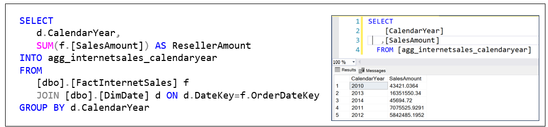
Figure 2 shows what an aggregation is. On the left is a SQL that creates the result on the right. It’s a table of the total Internet sales for each year, along with the count of the rows that comprise each total (SalesCount).

The total number of rows that were aggregated into the five rows is only about 60K, but we’re using a “sample/toy database”. In a real enterprise, there will be at least millions, up to billions and trillions of facts, depending on the nature of the data. For example, an e-commerce site could have just tens of thousands of individual sales, but another fact table might have tens of billions of captured Web page events (many more than just page clicks).

In any case, the results of the SQL in Figure 2 could be thrown away or persisted (written to a storage account/device) in case another query could make use of those results—that future query will not need to process potentially millions to trillions of rows again. For Kyvos, that persisted data is an aggregation. For this blog using SQL Server, it’s persisted as a materialized view.

Now, I realize the notion of a SQL GROUP BY and saving the results is ridiculously elementary. But as with many solutions (like LLMs), it begins with taking a simple, composable concept and scaling it to massive proportions.

Pre-Aggregation

That is basically what an aggregation is. However, the value of Kyvos over most current OLAP platforms is that those aggregations are created and persisted before any user has asked for them—known as MOLAP. That way, those aggregations aren’t created at the time of query, which would stall the return of the results—which wastes the time of the user and if it takes long enough, it can disrupt their flow of thought.

A good analogy is a well-stocked kitchen and pantry. Depending on our favorite meals, we would stock more or less of different things. Whatever we decide to cook, it’s a great benefit to have whatever we need right there, rather than having to take a trip to the store before and/or during the cooking process.

Like the old SSAS MD, Kyvos processes a set of aggregations, each a SUM and/or COUNT of a unique combination of attributes. Later in this blog, Abstract of Part 2 (preview of Part 2), I’ll talk a little about the many issues that can present themselves—it will make more sense later anyway.

For this blog, we’ll focus on aggregations themselves.

Pre-Agg, On-the-Fly Agg, Virtualization

But aggregations don’t just live in SQL queries. In OLAP systems, they come in different forms, each with their own trade-offs. OLAP solutions such as Kyvos support pre-aggregations, where summary data is materialized in advance from a root measure group at the lowest granularity. These are fast and stable but require configuration, processing time, and extra storage—yet another place to hold data.

Meanwhile, on-the-fly aggregations (kind of like ROLAP) are generated when needed, cached in memory, and vanish when the server restarts. At the far end is virtualization, which might not even use a dimensional model and instead stitches queries together across raw or federated sources.

On-the-fly aggregation still assumes a dimensional model—it simply calculates aggregations as queries come in. Virtualization, by contrast, often lacks a dimensional model altogether and may stitch together queries across disparate sources without any centralized schema.

Pre-aggregations have long been criticized for the burden of setup and maintenance. But techniques like partitioning help mitigate this by isolating “stable” data—data that probably won’t change—from “volatile” data, minimizing unnecessary processing. If all data is volatile, pre-aggregation is less useful and may not be worth the effort. On-the-fly advocates argue that users tend to stick to a narrow slice of a cube, so while the first query might be slow, subsequent ones hit cached aggregations and fly.

That might have worked when BI served relatively few (analysts, managers, data scientists). But thanks to data mesh, data vaults, and the rise of semantic layers, more data domains are entering the picture—and more knowledge workers are becoming BI consumers. As users explore across domains, cached aggregations won’t always help. In that reality, pre-aggregation scales better—preserving compute, handling concurrency, and serving a broader, less predictable spectrum of business questions.

In Part 2, we’ll dig into these OLAP trade-offs in depth—and why understanding them is critical as BI moves from departmental dashboards to enterprise-wide intelligence.

Materialized Views

Earlier, I mentioned my blog, All Roads Lead to OLAP Cubes… Eventually, gives you a good idea of the value of aggregations.

In “The Ghost of OLAP Aggregations – Part 2 – Aggregation Manager”, I discuss the orchestration that goes into high performance OLAP cube platforms such as Kyvos. But for now, let’s stick with this manual progression for that “behind the scenes” intuition.

The SQL in Figure 2 above could be referenced many times. The question of, “What is the total sales in 2010 (or 2011, etc.)?”, will pop up very often. We don’t need to keep re-executing that SQL across those billions to trillions of facts. Instead, we could cache it as a “materialized view”.

The concept of materialized views is implemented a little differently in various relational database platforms such as Oracle, Snowflake, and SQL Server. For simplicity, I’m just going to save the results of the SQL in Figure 2 as a table.

Figure 3 shows how we can save the SalesAmount totals by year into a table named agg_internetsales_calendaryear. The left is the SQL we’ll use. The right is the contents of the aggregate we just created.

Data More Than Five Years Old is Useless

As a reminder, the value of these aggregations is to minimize the querying of millions to trillions of facts. For many traditional OLAP implementations, the accumulation of that many facts is from extensive history. For example, an old and successful company like McDonalds or WalMart could have billions of sales per year, going back a few decades.

But it’s often argued that history beyond a few years old is useless for analytics. The world is rapidly changing and those patterns are obsolete. So, we store and process all that old data. We can archive it and analyze a smaller data set. Maybe we don’t need to worry about billions or trillions of rows.

I would still argue that it might not be the case for some industries where long-term trends provide great insights. Long-term trends may not predict the future, but they can help us understand how we got here, and so offer insights into fixing a current situation. It’s also important to remember that the volume of data has been growing exponentially over the past the decades. Meaning the last two years of data might be about as much as the prior decade. And, data is captured at a much lower granularity (more detailed), such as from web site visits to clicks, to even mouse movements!

Analytically valuable data isn’t just about history, the length of time we reach back to. It’s about spanning across space, the discovery of unknown and often unintuitive relationships between entities/concepts across those reaches. That means across wide breadths of data sources and across a wide population of BI consumers. I discussed this in my blog, Thousands of Senses.

Concurrency

The days of a handful of analysts, managers, and data scientists sending occasional heavyweight queries to a centralized BI platform are over. BI is no longer a specialist’s tool—it’s becoming embedded in the daily workflows of everyone.

Today, most knowledge workers—from nurses and logistics coordinators to warehouse staff and waiters—carry a mobile device capable of accessing insight-rich applications. These aren’t hypothetical use cases anymore. AI agents will increasingly query BI systems to supplement decisions in real time. Even IoT devices at the edge may reach into BI platforms to enrich local processing with broader trends or predictive context.

That means query concurrency is no longer an edge case—it’s the baseline. And this is exactly where pre-aggregation pays off. Every aggregation computed ahead of time means saved compute at query time, which scales far better across a wide, diverse, and growing range of BI consumers. Pre-aggregation isn’t just about speed—it’s about making BI viable for the masses.

Multiple Fact Tables

A dimensional data warehouse goes beyond just a single star schema as shown earlier in Figure 1. It’s a constellation of linked star schemas, each centered around a fact table, a log of a specific type. Figure 4 shows two fact tables linked through the DimProduct and DimDate dimensions.

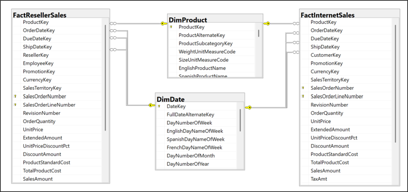
The left fact table, FactResellerSales, is a log of sales to resellers. The right fact table, FactInternetSales, is a log of sales to online customers. As shown, they have DimProduct and DimDate in common, but g=for simplicity, I left out the DimPromotion, DimCurrency, and DimSalesTerritory dimensions.

Note that FactResellerSales has an EmployeeKey but not FactInternetSales. Conversely, FactInternetSales has a CustomerKey but not FactResellerSales. This reflects the B2B and B2C nature of the FactResellerSales and FactInternetSales tables, respectively.

This hyper schema of linked star schemas enables us to analyze across different concepts and even domains.

Multiple Aggregations Per Query

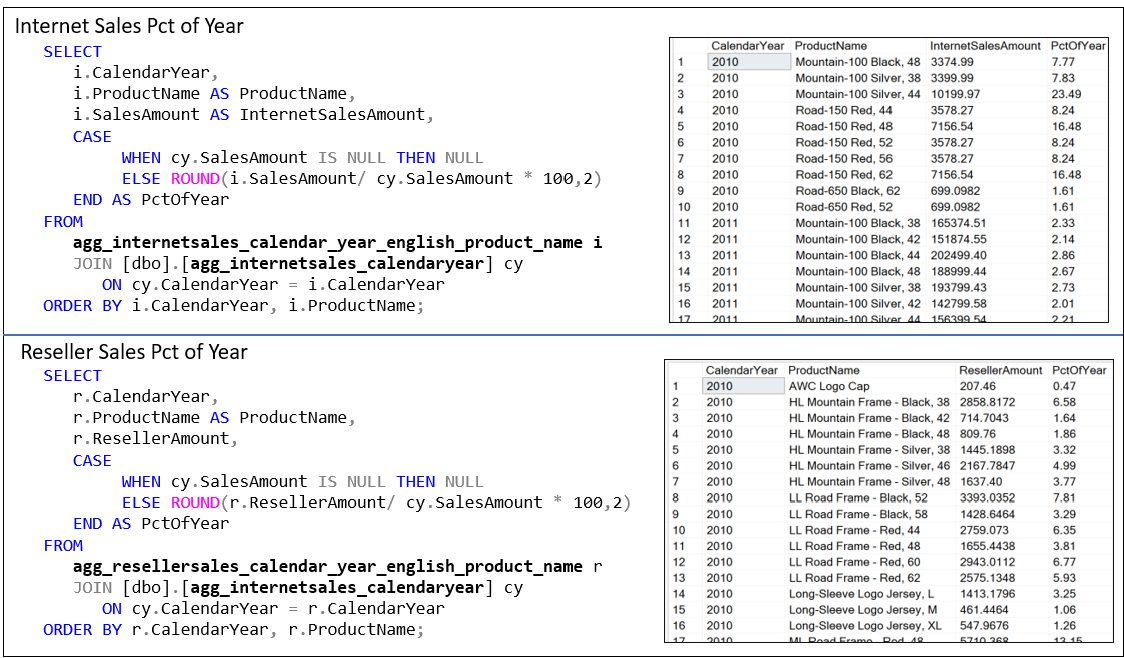
As mentioned, the “unit” question of OLAP is the slice and dice query. I call it the “unit” query because these slice and dice queries can be composed into more sophisticated, “higher-order” queries. For example, Figure 5 shows a SQL comparing the internet sales amount and reseller sales amount by year and product.

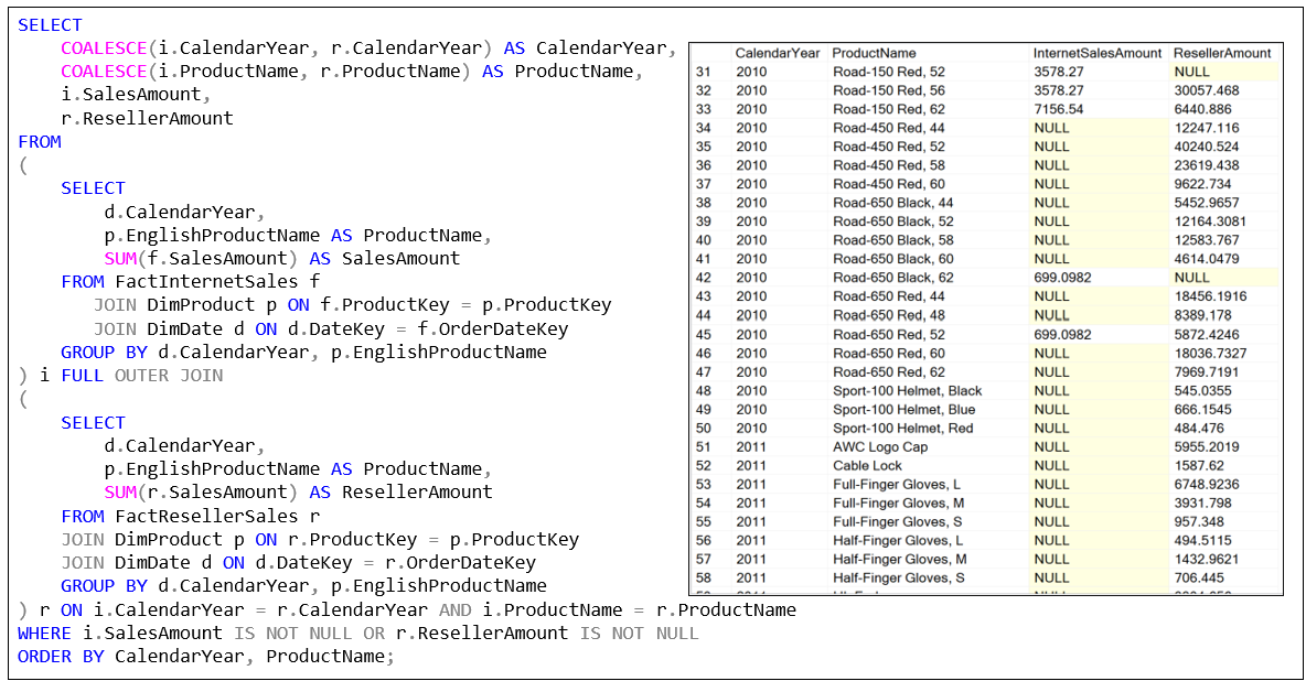
Note that the two fact tables can be very problematic with millions to trillions of rows. That runtime join of massive numbers of rows makes it worse that two separate aggregations. Of course, we can rewrite the SQL of Figure 5 for that purpose.

Figure 6 creates two aggregation tables that result in 271 and 568 rows.

Note that although the two SQL in Figure 6 create aggregations that are SQL tables (the INTO key word), the aggregations of an OLAP system (Kyvos, SSAS MD) are in a rather proprietary format optimized for fast reading (columnar, compressed, etc.). It’s close enough to compare it to Parquet—in fact, for some, it may actually be Parquet.

Figure 7 uses the two agg tables. Instead of integrating through what could be a table of billions of rows, it joins two substantially small tables that return the exact same results as Figure 5.

Lower Granularity Aggregation

The aggregations we created from the SQL in Figure 6 are at the calendar year and product granularity—one row for each product for each year. These aggregations are useful as long as our query requires information at that granularity.

But what if we want to slice and dice further? For example, Figure 8 shows a SQL diced by marital status as well as calendar year and product—granularity of calendar year, product, and marital status. Actually, the SQL also dumps the results into an aggregation shown on the right side named:

agg_internetsales_calendar_year_english_product_name_maritalstatus

Results versus Aggregations

The SQL query in the upper part of Figure 9 computes the percentage contribution of each product’s Internet sales to the calendar year’s total internet sales using already-aggregated data. While this specific output is useful for reporting or display—especially when formatted as a clean table showing PctOfYear—it is a point-in-time derivation. The result cannot be reused in other queries without repeating the logic or persisting the result somewhere, such as in a table or view.

In contrast, the two aggregations used in the query are far more reusable and flexible. These aggregated tables represent foundational metrics: one shows sales by product and year, the other shows total sales per year. Because these are clean GROUP BYs, they can be joined, filtered, or recombined for a variety of purposes—such as comparative analysis, trend calculations, or deeper drilldowns. They also avoid recalculating the same aggregations repeatedly. In contrast, the final result from the PctOfYear query is narrow in scope and doesn’t lend itself to easy reuse in other analytical contexts without restating the logic or nesting it within another query.

Additive Aggregations

At this point we’ve already created four aggregations. Questions should be arising as to what happens if we reach ten, twenty, even a hundred of them. Let’s hold those questions for Part 2, where I’ll cover the basics of the management side of OLAP aggregations.

For the moment, as a last exercise, let’s look at an example of the additive nature of aggregations (at least most of them). Let’s say we dropped the aggregation:

agg_internetsales_calendar_year_english_product_name

That aggregation is required for the SQL in Figure 7. Without that aggregation, but with the three remaining, will the SQL of Figure 7 be slow? It will still benefit from the aggregation broken down to a lower granularity with marital status:

agg_internetsales_calendar_year_english_product_name_maritalstatus

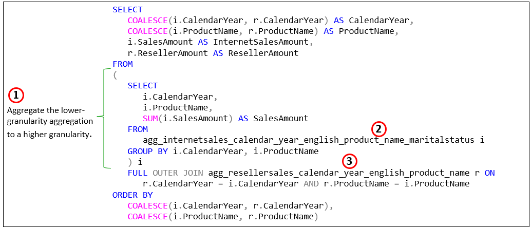
With that aggregation, we can derive the same values of the higher granularity aggregation: The sum of the marital status rows for each product equals the total for the product. Figure 10 below show what that SQL looks like:

1. This derived table aggregates the lower-granularity aggregation (product-year-marital) to the higher-level product-year.
2. The lower-granularity

As a reminder, it’s not that you, the user will create this SQL. This versatility is handled by the OLAP solution, as we’ll discuss in Part 2.

Abstract of Part 2

Just like that, we have four aggregations. But I think you get the gist of what aggregations are and their benefit. It’s a nice idea, but we can’t aggregate every single combination of attributes. A typical OLAP cube easily can consist of dozens of attributes across dates, customers, products, locations, employees, etc. We have only so much storage space and time to process, so we can really only aggregate a small percentage of possible attribute combinations.

A typical enterprise-class OLAP cube consists of dozens to hundreds of aggregations (a small percentage of the possibilities) to support a level of query performance that can range in magnitudes of gain. But not only is there only so much storage space and processing time, additionally something has to:

• Decide which aggregations will provide the most value.
  • That’s a moving target.
  • We can’t expect users (human, AI agent, or tool such as Tableau) to keep track of all the aggregations. Users should be able to construct a query as usual and have some system decide whether an existing aggregation .
• Maintain the aggregations. The thing about cache (aggregations are caches of compute) is that if something changes, it’s invalid. So, knowing when to recreate it is important.
  • Update the aggregations with new data.
  • Remove aggregations that aren’t worth the storage space and time to maintain.
• Have a backup plan when we don’t have a necessary aggregation.
  • Go to a “Plan B” at query time if a desired aggregation doesn’t exist, but there is one that can be utilized with minimal query time processing (i.e. a lower-granularity aggregation).
  • Go to a “Plan C” if no aggregation exists, even one we could use in an additive way. That is, calculate an in-memory aggregation on-the-fly.
• Explore and compare alternative approaches to the pre-aggregation of Kyvos and SSAS.
  • Includes on-the-fly aggregation, in-memory, materialized views.

Part 2 is about addressing the how of aggregations creation and effective utilization.

I should stress that the OLAP cube technologies (particularly Kyvos) are not just about aggregations and high query performance. They are also about presenting a user-friendly semantic layer—easy to understand and secured in an easily understood manner. I talk about this in Data Mesh Architecture and Kyvos as the Data Product Layer.

“Mr. Burn’s BI”, centered on OLAP cubes wasn’t superseded—no more than human-created functions were superseded by data science nor was data science superseded by LLMs. All are some of the components of an intelligenct enterprise platform. That’s in fact a big message of my book, Enterprise Intelligence, as I explain in my blog, Enterprise Intelligence: Integrating BI, Data Mesh, Knowledge Graphs, Knowledge Workers, and LLMs

Notes

• This blog is Chapter VIII.4 of my virtual book, The Assemblage of Artificial Intelligence.
• Time Molecules and Enterprise Intelligence are available on Amazon and Technics Publications. If you purchase either book (Time Molecules, Enterprise Intelligence) from the Technic Publication site, use the coupon code TP25 for a 25% discount off most items.