Contents
Enterprise Intelligence
- What are “Insights” (in the context of Enterprise Intelligence)?
- Tips for Auto-Seeding a new EKG
- Why bother with BI in this era of LLM-driven AI, Spark, and cloud data warehouses?
- How is the TCW System ⅈ probing optimized?
- Is there a List of Interesting videos and articles that support the concepts in Enterprise Intelligence?
- What Do You Mean by “Knowledge is Cache”?
- Support Vector Machine Build Cost
Semantic Web / Knowledge Graph
- Baby Step for Incorporating the Semantic Web into BI
- How can you be a Good wikidata.org Citizen?
- LLM–Knowledge Graph Symbiosis
Business Intelligence in an AI World
- What is pre-aggregation in OLAP?
- What is the importance of SQL GROUP BY statements?
- What is the difference between OLAP, cubes, and semantic layer?
- How to Handle Client-Side Calculations in the Age of AI.
- What Does BI Do So that AI Agents Don’t Need to Worry About It?
- 50 Innovations BI history provides
Time Molecules
- What are the Three Time-Based Relationships of Time Molecules?
- Isn’t Time Molecules just Process Intelligence?
Artificial Intelligence
- What’s the difference between a tuple and a vector? Can a tuple ever be a vector?
- Should we use a private LLM?
- What are chunk size guidance for vector database embeddings?
Architecture
- What is a Data Vault and a Business Vault?
- What is the Difference Between ETL and ELT?
- What is the Difference between Process, Business, and Operational Intelligence?
What’s the difference between a tuple and a vector? Can a tuple ever be a vector?
All vectors are tuples, but only purely numeric tuples (with vector-space operations) are vectors.
- A tuple is simply an ordered list of elements, which can be of any type (numbers, strings, dates, labels, etc.).
- Example:
("Bikes", 2025, 5000)is a 3-tuple, but you can’t add or scale it because “Bikes” and “2025” here are non-numeric labels.
- Example:
- A vector is an ordered list of numeric values (elements from a field) equipped with well-defined addition and scalar-multiplication operations that satisfy the vector-space axioms.
- Example:
(5000, 3000, 12.5)is a 3-vector in ℝ³—you can add two such vectors, multiply by scalars, compute dot-products, and measure distances.
- Example:
- Overlap: Every numeric vector is also a tuple (an ordered list), but not every tuple is a vector. A tuple only becomes a vector when:
- All components are numeric, and
- You define how to add two tuples and multiply them by scalars (the standard component-wise operations).
What is pre-aggregation in OLAP?
Pre-aggregation means computing and storing summaries (e.g. sums, counts, averages) of your detailed fact data ahead of time—across various combinations of dimensions—so that analytic queries can read those summaries instantly instead of scanning millions (or billions) of raw rows at query time. See The Ghost of OLAP Aggregations – Part 1.
Update (March 3, 2026)
I’d like to clarify some terminology used in this post. When I refer to “OLAP cubes”, I’m specifically highlighting the multidimensional data structure optimized for analytical queries—distinct from relational databases traditionally geared toward OLTP (Online Transaction Processing) patterns. Kyvos originally built on this OLAP foundation for high-performance analytics at scale (ca. 2015). However, the Kyvos platform has since evolved into a comprehensive semantic layer that delivers a unified, consistent business view across disparate data sources—ensuring “one view, one meaning” for metrics, dimensions, and relationships enterprise-wide. This semantic model retains the core acceleration structures for query speed and efficiency—even more valid today as multiple factors expand the need for trusted data—while expanding to support modern AI-driven insights, data mesh, and enterprise intelligence frameworks. OLAP described how it accelerated analytics. Semantic model describes what it represents. For the latest on Kyvos, check their official resources at kyvosinsights.com.
Why use pre-aggregation?
- Performance: Drastically speeds up complex queries (e.g., month-to-date sales by product and region) by hitting small summary tables instead of the full fact table.
- Scalability: Supports interactive slicing, dicing, drilling, and pivoting over large datasets without taxing your database.
- Concurrency: By serving queries from small aggregate tables, the system avoids heavy compute on the base fact, allowing many users to query simultaneously without contention.
- Predictability: Provides consistent query response times—even as data volumes grow.
How do OLAP engines (SSAS, Kyvos) implement pre-aggregation?
- SQL Server Analysis Services (SSAS):
- Uses Aggregation Designs to pick dimension hierarchies and measure groups.
- Builds multi-level aggregate tables inside the cube (stored in MOLAP or ROLAP storage).
- Supports usage-based optimization—profiles query patterns, then dynamically refines which aggregates to build.
- Offers incremental process so only changed partitions rebuild aggregates.
- Kyvos Analytics:
- Creates distributed cubelets on Hadoop or cloud storage, each holding pre-aggregated slices.
- Leverages a massively parallel engine to shard aggregates across nodes.
- Uses dynamic aggregate pruning to only read relevant cubelets per query.
- Integrates with modern data lakes for on-demand aggregate re-calculation without full cube reloads.
What’s the trade-off?
- Storage Cost: More disk space for summary tables or materialized views.
- Load Time: ETL must compute and refresh aggregates (batch or incremental), adding complexity.
- Flexibility: Ultra-detailed ad-hoc queries outside pre-defined aggregations may still hit the raw data or require on-the-fly aggregation.
Pre-Aggregation vs. On-The-Fly Aggregation
| Aspect | Pre-Aggregation | On-The-Fly Aggregation |
|---|---|---|
| Query Speed | Instant (reads precomputed data) | Slower (scans raw data) |
| ETL Complexity | Higher (build & maintain summaries) | Lower (no extra ETL) |
| Storage Footprint | Larger (additional summary tables) | Minimal (only raw fact tables) |
| Flexibility | Limited to defined cubes/views | Fully flexible but slower |
When should I use pre-aggregations?
- High-volume analytics where sub-second response is critical.
- Repeatable reporting patterns (e.g. monthly, quarterly dashboards).
- Interactive BI tools that expect instant pivots and drill-downs.
Example
1. Base fact table (billions of rows)
Schema: FactSales(OrderDate, Product, Region, Sales)
| OrderDate | Product | Region | Sales |
|---|---|---|---|
| 2025-01-01 | Bikes | North America | 120 |
| 2025-01-01 | Cars | Europe | 340 |
| … | … | … | … |
| 2025-12-31 | Bikes | Asia | 215 |
| 2025-12-31 | Cars | North America | 480 |
That single table might hold 5 billion rows—too large for sub-second ad-hoc queries.
2. Pre‐aggregation designs
Below are a few of the aggregate combinations we build ahead of time:
| Agg Name | Dimensions | Measures | Grain |
|---|---|---|---|
| Year_Product | Year | SUM(Sales) | (2025, Bikes) |
| × Product | COUNT(*) | (2025, Cars) | |
| Year_Region | Year | SUM(Sales) | (2025, North America) |
| × Region | (2025, Europe) | ||
| Product_Region | Product × Region | SUM(Sales) | (Bikes, Asia) |
| (Cars, Europe) |
3. Query flow
- Lookup pre-agg: When you ask
SELECT SUM(Sales) FROM FactSales WHERE YEAR(OrderDate)=2025 AND Product='Bikes', the engine checks the Year_Product aggregation first. - Hit → returns the pre-computed SUM in milliseconds.
- Miss → if you queried a combination not covered (e.g. Year+Region+Product), it either:
- Falls back to on-the-fly aggregation over FactSales (slower), or
- Remaps to a closest pre-agg plus a small roll-up if supported.
4. Why it works
With a well-designed set of pre-aggregations that match 80–90% of your common query patterns, the OLAP engine “hits” the right aggregate table most of the time—delivering interactive performance on billion-row datasets.
What are “Insights” (in the context of Enterprise Intelligence)?
Insights refer to the salient patterns, anomalies, relationships, and metrics observed by business users while exploring visualizations generated from BI query results. These visualizations—such as bar charts, line graphs, scatter plots, and heatmaps—serve as the lens through which human users detect meaningful observations.
Insights include, but are not limited to:
- Inflection points (where growth or decline changes pace)
- Trends and seasonality
- Outliers and anomalies
- Inequality metrics such as the Gini coefficient
- Correlations or clusters
- Unexpected gaps or spikes
Some insights may be obvious to one user but missed entirely by another—a phenomenon akin to a “Where’s Waldo” effect. Others may not seem relevant to the current viewer but may prove valuable when surfaced to different stakeholders or intelligent agents (AI).
In an Enterprise Intelligence framework, insights are not just ephemeral “aha” moments. Instead, they are captured, stored, and made discoverable—creating a shared memory of intelligence that can be reused, validated, or built upon by others across the organization. This collective intelligence can support:
- Better decision-making across teams
- Cross-domain collaboration
- AI-driven automation and recommendations
Ultimately, insights are the reason BI analysts use visualization tools in the first place. They represent the bridge between data and action—the distilled value from the mountain of raw metrics that flow through the BI system.
What are the Three Time-Based Relationships of Time Molecules?
Time is the ubiquitous dimension. Without it, nothing happens—there are just things, not processes. So in the world that is constantly changing, undermining what we’re learned, we rebuild our understanding by observation. These are three ways that we observe what’s going on.
- Markov Models – “What happens next?”
At the process level, we look at sequences of events across many instances (cases) of a process.- Question: Given the last event, what is the next event?
- Example: In a customer support process, after “Ticket Assigned,” the next event might be “Ticket Resolved” 65% of the time, “Customer Follow-up” 25%, and “Escalated” 10%.
- This captures transition probabilities between events of a process.
- Conditional Probabilities – “Under these conditions, how likely is it?”
We focus on context: given certain conditions or accompanying events, what is the probability a particular event will occur?- Question: Given a set of circumstances, how likely is a given event?
- Example: “Given that the customer is VIP and the ticket priority is High, the probability of escalation is 45%.”
- This reflects the idea of what fires together, wires together — associations strengthened by repeated co-occurrence.
- Correlations – “Do these things move together over time?”
Here, we measure how two variables or event measures rise and fall together over increments of time.- Question: How closely do two different metrics track each other over time?
- Example: Weekly call volume and average customer wait time might have a correlation of 0.82, suggesting a strong positive relationship.
- This doesn’t prove causation but can point to potentially related behaviors or metrics.
How they connect
Markov Models (1) and Conditional Probabilities (2) together form the two halves of a Hidden Markov Model (HMM) — the transitions between states (Markov) and the probabilities of observed events given those states (Conditional).
Correlation (3) operates alongside them as a discovery mechanism, hinting at relationships worth testing or modeling. See Correlation is a Hint Towards Causation.
Isn’t Time Molecules just Process Intelligence?
Date added: March 15, 2026
Roughly, there is significant overlap. But my approach and prime interests are different.
When I began writing Time Molecules in mid-2024, I was not thinking in terms of “Process Intelligence” as a known category. I had checked around, and at least in my world—mostly BI and data people—the term was mostly unknown (very surprising in hindsight). What I did see was the process mining world expanding beyond pure process discovery and conformance checking into richer analytics. My impression at the time was that it was still getting there.
My own motivation for Time Molecules came from a somewhat different direction.
One of the core ideas was that time is the most ubiquitous dimension in the enterprise. It is the one dimension that can relate just about every database, because almost everything that matters in a business happens over time. Sales happen over time, customer interactions happen over time, shipments happen over time, machine telemetry happens over time, web activity happens over time, and increasingly, AI agent activity happens over time as well.
That made me think there was room for something broader than traditional BI and somewhat different in emphasis from classic process mining—the time-side of thing-oriented BI.
Time Molecules was meant to address a world in which:
- IoT devices were generating more event streams.
- AI agents would increasingly become participants in business processes.
- More knowledge workers would be plugged into enterprise systems through mobile devices and other always-connected interfaces.
- Business Intelligence would need to expand beyond static measures and dimensions into recurring patterns of behavior through time.
So while there is certainly overlap with process mining and with what is now often called Process Intelligence, my original purpose was not simply to repackage those ideas.
My aim was more specifically to bring process-pattern thinking into the BI and enterprise intelligence world.
Traditional BI has been strongest at analyzing things: sales, costs, products, customers, regions, KPIs, and trends. But businesses are not made only of things. They are also made of stories: recurring sequences of events, delays, loops, handoffs, decisions, and outcomes. I saw Time Molecules as a way to make those stories into first-class analytic structures.
That is one reason the subtitle referred to the BI side of process mining and systems thinking. My emphasis was less on an operational control tower and more on integrating process behavior into the broader intelligence of a business. In my mind at the time, process mining leaned more operational, while BI leaned more tactical and strategic. I knew all of these could span operational, tactical, and strategic uses, but the center of gravity seemed different.
It would be close to say “Time Molecules is just Process Intelligence”. But, from my intent, a fairer way to say it is this:
- Process Intelligence often emphasizes operational visibility and action
- Time Molecules was aimed at making time-oriented process behavior part of Business Intelligence and is an extension to my other book, Enterprise Intelligence.
It was an attempt to treat temporal patterns almost as the counterpart to the thing-oriented structures of traditional BI.
As I wrote in Time Molecules:
Ultimately, Time Molecules builds on the foundation of Enterprise Intelligence by focusing on the dynamic, evolving nature of processes within the enterprise. Combining event sequences, conditional probabilities, and process-centric models shifts the focus from static data analysis to a fluid, interconnected view of the intelligence of a business.
That still captures the heart of it for me.
And today, my push on Time Molecules is increasingly within the broader Assemblage of AI framework, where event streams, processes, agents, probabilities, and enterprise intelligence all come together in a larger architecture.
So while I now recognize the overlap with Process Intelligence more clearly than I did in 2024, I still see Time Molecules as having had a distinct mission. That is helping the BI world think in terms of time, process, and the evolving intelligence of a business.
Please see this blog which explains Time Molecules based on the Bi world.
Support Vector Machine Build Cost
An SVM gives us a quantitative border to measure “how far we can push,” but it’s heavier than the usual linear/stat functions (SUM/AVG, inflection points, Markov models). Two practical points:
- Training vs serving.
A linear SVM is light to train and very cheap to serve (just a dot product per row). A kernel SVM (e.g., RBF, curved borders) can be slow to train and costlier to serve because it depends on many support vectors. OLAP cubes help by delivering the training slice fast, but model fitting is still the expensive step. - Build on demand, then re-use.
When a boundary question is new (features/slice not seen before), the agent can approve a build. We submit it to a background pipeline, cache the model as an Insight Space Graph model (tied to the QueryDef, feature list, scaler, and data slice), and serve it immediately on future queries. That turns a one-time heavy compute into a reusable asset.
Implementation rules of thumb:
- Default to linear SVM for most BI use cases—fast to fit, tiny artifact (store just weights/bias), exact margins for “allowable Δ.”
- If curvature is clearly needed, allow kernel SVM or a kernel approximation so serving stays near-linear.
- Prefer margins over calibrated probabilities in real time; probability calibration can run in the background.
- Version and expire models based on data freshness (batch/window), so cached borders track the underlying cube.
The first time may take longer, but after that the SVM becomes part of the ISG, ready to answer “how far can I push?” or “what’s the minimal change to reach state 8?” with near-instant latency.
LLM–Knowledge Graph Symbiosis
A symbiotic relationship between Large Language Models (LLMs) and Knowledge Graphs (KGs) arises when each compensates for the other’s weaknesses while amplifying the other’s strengths.
- LLMs excel at fluid reasoning and contextual synthesis. They can interpret natural language, infer intent, and generalize from incomplete information. However, their knowledge is implicit, approximate, and decoupled from provenance—they recall patterns but cannot guarantee truth.
- Knowledge Graphs, on the other hand, hold explicit, structured truth. They define entities, relationships, and ontologies that are verifiable and contextualized, but are static and brittle without external interpretation.
In combination, the LLM becomes the context engine—the conversational and interpretive front end—while the Knowledge Graph becomes the semantic ground truth that anchors responses and decisions. The LLM retrieves and composes meaning from the KG, and the KG in turn gains new inferred links, entity definitions, and natural-language descriptions from the LLM’s interpretive feedback.
This is a bi-directional learning loop:
- The LLM queries the KG to constrain its imagination with reality.
- The KG absorbs insights from the LLM to expand its ontology with newly discovered or reformulated relationships.
In practical terms, this symbiosis mirrors the human balance between intuition and memory. The LLM acts like the right hemisphere—pattern-oriented, associative, creative—while the Knowledge Graph acts like the left hemisphere—structured, logical, and archival. The result is not merely retrieval-augmented generation (RAG), but a continuously evolving hybrid intelligence capable of both contextual understanding and logical consistency.
See “Symbiotic Relationship between KGs and LLMs”, page 94 in Enterprise Intelligence.
Baby Step for Incorporating the Semantic Web into BI
If you’re new to knowledge graphs and the Semantic Web, I wrote a page on a baby step towards incorporating the Semantic Web into your BI platform. It was intended to be an appendix in Enterprise Intelligence, but missed the cut. This baby step will take you from:
- Acquainting yourself with knowledge graphs through playing with Wikidata.org and playing with SPARQL using Wikidata’s query tool.
- Introduction to Semantic Web terms—SPARQL, RDF, OWL, IRI …
- Selecting a platform – I recommend Jena Fuseki as the open source graph database, Stanford’s Protege as a visualization tool.
- Retrofitting your BI database for the Semantic Web.
- An MVP for BI visualizations—as discussed in Enterprise Intelligence, Contextual Information Delivery, page 284. Figure 1 shows the associated snapshot from the book, Figure 100 on page 285.
Next baby step: Tips for Auto-Seeding a new EKG
Why bother with BI in this era of LLM-driven AI, Spark, and cloud data warehouses?
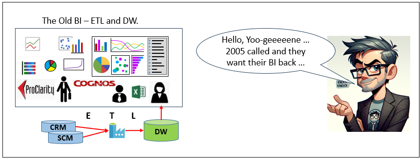
In today’s AI discourse, Business Intelligence can feel like legacy infrastructure—associated with slow cubes, brittle ETL, and static warehouses. But that framing overlooks what BI actually represents architecturally: the enterprise’s most curated, trusted, and decision-ready data substrate. BI integrates domain data, harmonizes terminology into a shared business language, enforces governance, and presents information in interpretable dimensional models designed for human and machine consumption alike.
Modern AI systems actually amplify the need for the curation of BI. LLMs, agents, and machine learning pipelines are only as reliable as the data they reason over. Without curated semantic layers and governed data products, AI operates on fragmented, inconsistent signals. Contemporary patterns such as Data Mesh, Data Vault, and cloud-scale warehousing have already evolved BI beyond its monolithic past, while AI now helps stitch distributed domains back into coherent knowledge systems rather than replacing them.
BI is the art and science of transforming raw data to a humanly intuitive level of abstraction.
There is also a cognitive analogy. Human intelligence does not reason directly over raw photons, sine waves, or molecular signals. Early sensory processing (such as visual cortex transformations) converts raw input into higher-order constructs the brain can interpret and reason about. BI plays a similar role for the enterprise—transforming operational exhaust into structured, decision-grade information. For this reason, even in an AI-driven architecture, BI remains the spearhead of enterprise intelligence: not antiquated infrastructure, but the curated substrate upon which reliable machine reasoning depends. See Thousands of Senses.
At Kyvos Insights, where I work as Principal Solutions Architect, we build exactly this, a universal semantic layer that unifies data sources into one governed business view with consistent metrics, hierarchies, and logic—delivering sub-second queries even at massive scale. It preserves BI’s hard-earned curation while grounding AI agents and LLMs in trusted context, cutting hallucinations and enabling reliable, explainable decisions. See how it works at kyvosinsights.com.
What is the importance of SQL GROUP BY statements?
A GROUP BY is a foundational SQL construct used to aggregate detailed data into summarized form. It partitions rows in a fact table into groups based on one or more shared dimension values, then computes metrics (aggregations) for each group.
In Business Intelligence and OLAP query patterns, GROUP BY statements are among the most common query forms because they transform raw transactional data into analytically meaningful structures suitable for reporting, visualization, and correlation analysis. It’s the query pattern that addresses the fundamental slice and dice query.
Example:
SELECT Customer, SUM(Sales) AS TotalSalesFROM FactSalesGROUP BY Customer;
This query summarizes total sales per customer.
Parts of a GROUP BY query
- SELECT (dimension columns): The categorical fields that define how data is partitioned (e.g., Customer, Product, Region).
- SELECT (aggregation functions): Metrics computed for each group (e.g., SUM, COUNT, AVG, MIN, MAX, STDEV).
- FROM (source table or fact table): The dataset being summarized, typically a transactional or event-level table.
- GROUP BY clause: The instruction that partitions rows into groups sharing identical dimension values.
- Optional filters (WHERE / HAVING): WHERE filters rows before grouping; HAVING filters groups after aggregation.
Result structure
The output of a GROUP BY query is a summarized tabular dataset (dataframe):
- Each row represents one unique combination of the grouped dimensions.
- Each row therefore constitutes a tuple—a context-bound data record defined by its dimensional coordinates and associated aggregated metrics.
Why it matters in OLAP patterns
GROUP BY queries:
- Produce dimensional summaries used in dashboards and reports
- Form the basis of cubes and semantic models
- Generate tuples that can feed correlation, trend, and process analyses
In analytic architectures, GROUP BY is the primary mechanism for transforming granular events into structured insight artifacts.
What is the chunk size guidance for vector database embeddings?
There isn’t one magic word-count, but there is a sweet spot—and it’s better to think in tokens than words.
Practical targets (what usually works)
- 128–256 tokens (≈ 90–180 words)
Best when you want precise retrieval: definitions, facts, “where is the one sentence that answers this?” - 256–512 tokens (≈ 180–360 words)
Best general-purpose default: enough context to be interpretable, still specific enough to retrieve cleanly. - 512–1024 tokens (≈ 360–750 words)
Best when answers require broader context (policies, multi-paragraph explanations, “what does this section mean?”).
Rule of thumb: start around ~300–500 tokens (≈ 200–350 words) for “knowledge chunks,” then adjust based on what your queries look like.
When it’s too little vs too much
- Too little: chunks are so short that they lose the “why/which/under what conditions” context, so retrieval pulls fragments that don’t stand alone.
- Too much: chunks contain multiple topics, so a query matches something inside, but the returned chunk is noisy and the LLM has to hunt.
What is the different between OLAP, cubes, and semantic layer?
Many people who have been around BI and data warehousing for at least a decade might use OLAP, cubes, and semantic layer interchangeably. They’re not the same thing.
- OLAP was the breakthrough that let us analyze data interactively instead of waiting for reports. It gave us multidimensional thinking: measures, hierarchies, drill paths, aggregation awareness.
- OLTP is about transactions. It’s optimized for inserts, updates, and row-level lookups. Relational databases excel at this. Relational systems were designed for OLTP workloads.
- OLAP is about analytical query patterns. It’s optimized for aggregations, scans, grouping, drilldowns, and multidimensional exploration across large volumes of data. OLAP introduced data structures and access patterns specifically engineered for analytics.
- Cubes were the performance engine. They pre-computed aggregates, enforced business logic, and delivered sub-second response times at scale. They weren’t just storage structures—they were governance and acceleration combined.
- Semantic layers abstract business meaning from physical data. They define metrics, dimensions, relationships, and rules so every consumer—BI tools, SQL users, applications, and now AI agents—gets consistent answers.
- A modern semantic layer doesn’t eliminate OLAP or cube principles—it incorporates them. It operationalizes decades of BI discipline into a governed, scalable architecture that serves both humans and machines.
The relevance of these terms is still critical today for the application of AI in the enterprise. Today, the number of BI consumers is exploding:
- AI agents are querying data alongside humans.
- Self-service analytics continues to expand.
- IoT, including telemetry from mobile apps used by knowledge workers, is multiplying both data sources and event volumes.
The presence of AI does not reduce the need for BI discipline. If anything, it amplifies it. When agents generate queries at scale, consistency, aggregation awareness, and governed definitions become even more essential.
That growth in queries isn’t just about the speed required for AI agents, but the ability to take on the new levels of query concurrency. More consumers means more simultaneous queries.
When the data structures are intelligently designed and materialized, you don’t just reduce query latency, but the reduced compute resulting in faster query speed can be used to handle higher query concurrency. You avoid repeated full scans. You prevent contention. You create headroom for hundreds or thousands of concurrent semantic-layer consumers.
Pre-aggregation provides both performance and scalability.
Kyvos has evolved far beyond our roots as a traditional cube platform. Today, Kyvos is a semantic layer built on OLAP principles—not a legacy cube product, but a cloud-native architecture that embeds aggregate awareness, governance, and performance into the semantic tier itself.
In the AI era, the semantic layer isn’t just about consistent metrics. It’s about delivering governed, sub-second answers — reliably — to an ever-growing population of human and machine analysts.
The future isn’t replacing OLAP principles, rather applying them at cloud scale.
What is the Difference between Process, Business, and Operational Intelligence?
| Aspect | Business Intelligence | Operational Intelligence | Process Intelligence |
|---|---|---|---|
| Main focus | Business performance | Current operations | Flow of work over time |
| Core question | What happened and how are we performing? | What is happening right now? | How did this unfold? |
| Typical time horizon | Historical and trend-based | Real-time or near-real-time | Historical or near-real-time across a case |
| Primary unit of analysis | KPIs, measures, dimensions | Live events, alerts, statuses | Cases, paths, transitions, durations |
| Typical data shape | Aggregated facts and dimensions | Event streams, telemetry, queues, logs | Event sequences tied by case ID |
| Typical outputs | Dashboards, scorecards, reports | Alerts, monitoring views, live operational dashboards | Process maps, bottlenecks, branching, conformance views |
| Example question | Which region had the lowest margin last quarter? | Which machines are failing right now? | Where do cases most often stall or loop? |
| Main users | Executives, managers, analysts | Operations teams, supervisors, responders | Process owners, analysts, operations leaders |
| Decision style | Strategic and tactical | Immediate and reactive | Improvement and redesign |
| In your architecture | Aggregates events into business facts | Watches events as they happen | Reconstructs event stories from events |
