An MDX Primer

Previously, on The Ghost of MDX …

This post is Part 2 of my prior post, The Ghost of MDX (Multi Dimensional eXpressions), where I discussed the value of pre-aggregated OLAP, such as SQL Server Analysis Services and Kyvos SmartOLAP, in the modern Cloud world.

Before continuing, I need to clarify that by “SQL Server Analysis Services” (SSAS), I’m referring to the older “multi-dimensional” edition (SSAS MD). That is, as opposed to the newer “Tabular”, in-memory edition or its Cloud-based equivalent called “Azure Analysis Services”.

Here in this post, I’d like to take a small step towards removing some of the mystery around MDX. I hope to teach you a few things I wish I knew when I started with MDX over 25 years ago. It’s my claim that MDX is an elegant language that isn’t really hard to learn. That is, if you know the things I wish I knew when I first learned MDX–when I was thrown into the deep end during that indescribably tough crunch-time months before the release of SQL Server 7.0 back in November 1998–on the job, without even knowing what an “OLAP” was, and everyone else too busy to help while scrambling towards the big deadline.

My intent is to simply break the ice in your quest to learn MDX, or to better understand what it all really means beyond something you cut/paste from StackOverflow and modify. Why would you want to do something crazy like that? Because the notion of high-dimensional space is manifesting in a big way today as vectors embeddings (a core of LLMs), hyperparameter optimization in machine learning (searching the space of optimal values), and the recognition of linear algebra itself as the prime math skill in machine learning. MDX’s middle name is “multi-dimensional”, after all.

We will not “learn” MDX in this blog, but hopefully it will be easier with available comprehensive material. I think the best book for learning MDX is MDX Solutions, by George Spofford.

Challenges for SQL Experts Transitioning to MDX

People with extensive experience in SQL often face initial struggles when transitioning to MDX because they look similar from a distance, but the data structures they query are fundamentally different. MDX was designed to look somewhat like SQL because it was logical to assume that new cube developers would come from the relational database management system (RDBMS) world. Ironically, the superficial similarity in syntax can be misleading and confusing. Here’s why:

Nature of Data Structures

• SQL: In SQL, data is typically represented as a one-dimensional array of tuples. Each row in a table or result set is essentially a list of tuples. You’re probably vehemently arguing that SQL results are 2D. But it really is a list (a 1D structure) of objects made from the columns of the table.
• MDX: In contrast, MDX operates on multidimensional structures called cubes. The results of an MDX query, known as a cellset, are truly multidimensional arrays of values. This means that the SELECT part of an MDX query defines the axes (e.g., rows, columns, pages) rather than just columns.

SELECT Clause

• SQL: The SELECT statement in SQL is used to specify the columns to be retrieved from a table. It selects data from one or more tables and presents it in a tabular format.
  • Example: SELECT column1, column2 FROM table WHERE condition;
• MDX: The SELECT statement in MDX defines the axes of the cellset. Instead of specifying columns, it sets the dimensions for the rows and columns in the result set.
  • Example: SELECT { [Measures].[Sales] } ON COLUMNS, { [Date].[Year].[2020] } ON ROWS FROM [SalesCube];
  • In this example, [Measures].[Sales] is placed on the columns axis, and [Date].[Year].[2020] is placed on the rows axis.

WHERE Clause

• SQL: The WHERE clause in SQL filters rows based on Boolean conditions. It determines which rows of data will be included in the result set.
  • Example: SELECT * FROM table WHERE column1 = 'value';
• MDX: The WHERE clause in MDX, also known as the slicer axis, sets a context that overrides the default members of all attributes in the cube that are not referenced in any axis. It does not filter rows but instead slices the data to focus on a specific subset.
  • Example: SELECT { [Measures].[Sales] } ON COLUMNS, { [Date].[Year].[2020] } ON ROWS FROM [SalesCube] WHERE ([Geography].[City].[New York]);
  • In this example, the slicer axis [Geography].[City].[New York] sets the context for the query, focusing on sales data specific to New York City.

WITH Clause

• SQL: The WITH clause in SQL is used for Common Table Expressions (CTEs), which define temporary tables within the scope of a SELECT, INSERT, UPDATE, or DELETE statement. These CTEs make queries more readable and maintainable by breaking them into logical parts.
  • Example: WITH cte AS (SELECT * FROM table WHERE condition) SELECT * FROM cte;
• MDX: The WITH clause in MDX is used to define calculations, sets, members, or tuples. These defined objects can then be used within the query to create complex calculations and retrieve specific subsets of data.
  • Example: WITH MEMBER [Measures].[Profit] AS ([Measures].[Sales] - [Measures].[Cost]) SELECT { [Measures].[Profit] } ON COLUMNS FROM [SalesCube];
  • In this example, a new member [Measures].[Profit] is defined, which calculates the profit by subtracting cost from sales, and this new member is then used in the SELECT statement.

The fundamental differences in data handling, the roles of the SELECT and WHERE clauses, and the usage of the WITH clause in SQL and MDX are key areas where SQL experts may initially struggle. Understanding these distinctions is crucial for effectively transitioning from SQL to MDX and leveraging the full potential of multidimensional data analysis.

An MDX “Hello World” – “SELECT cust_ID, cust_name FROM customers”

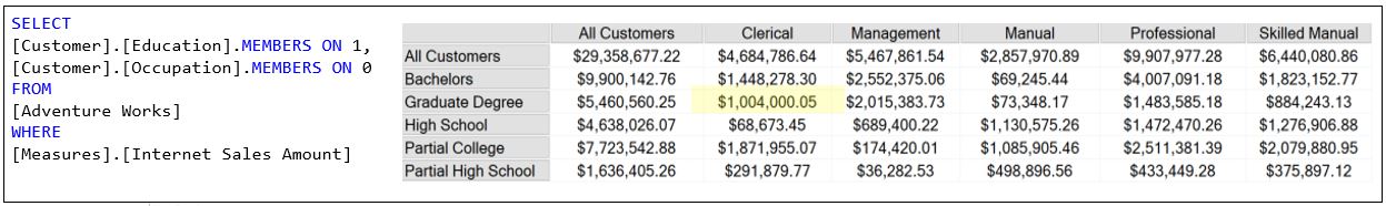
Let’s start out by dissecting a very basic MDX. Figure 1a illustrates a very simple MDX querying the AdventureWorks2017 SSAS OLAP cube.

Here is a description of what is depicted in Figure 1a in plain English:

On the rows are the Education Levels. On the Column are Occupation Types. The values are Internet Sales Amount for each combination of Education Level and Occupation Type. Further, this only includes internet sales for bikes during the year of 2013.

Figure 1b is the result I’ve copied to Excel with a few enhancements. It’s a 2-dimensional grid filled with values.

Notice along the left side, top, and bottom of Figure 1b are fragments that map to the MDX shown in Figure 1a. So let’s restate what we see in Figure 1b, but using MDX terminology:

1. Axis 0 is comprised of the set of Occupation Levels of the Customer dimension.
2. Axis 1 is comprised of the set of Education Levels also from the Customer Dimension.
3. The cells are the Internet Sales Amount for each tuple comprised of a member from the Occupation Level and Education Level axes.
4. The results are sliced by the Bike member of the Category attribute of the Product dimension and the year 2013 of the Calendar Year attribute of the Date dimension.

I’ll now briefly define the highlighted jargon – dimension, member, tuple, set, attribute – as well as value and subcubes.

Dimension, Attribute, Hierarchy

For a software application that’s called “multi-dimensional”, “dimension” is a very important word. However, it’s a source of confusion right off the bat.

“Dimension” doesn’t have the same meaning as you’d think, like when we’re talking about geometry, linear algebra, or physics. In SSAS, “dimension”, should really be called “entity”. For example, in AdventureWorks, there is the Customer entity, the Product entity, the Date entity, etc.

Figure 2 shows examples of dimensions (1), attributes (2), and hierarchies (3) in the AdventureWorks data warehouse. The left side of Figure 2 (1) shows that there are 17 “dimensions” – which should be called entities – in the AdventureWorks cube. (Don’t count the AdventureWorks and KPI nodes.)

Each entity consists of a number of attributes (2). That is, things that describe each entity. For example, a customer has among other things name, address, and gender attributes. Or product entities having ISBN, price, and category.

The concept of dimension in the geometric sense are really attribute and level. Each attribute and level in an SSAS cube is a dimension of the cube. Additionally, the measures of a cube are grouped into a “Measures dimension” as well.

Hierarchies (3) are an ordered set of attributes. Hierarchies categorize attributes. For example, the Customer dimension has a [Customer Geography] hierarchy of Country, State, City, Postal Code, and finally all the customers. But in Figure 2, we see the more familiar date hierarchies.

Members

Members are the individual points or elements within an attribute of an OLAP cube. They are the “labels” on each axis of the cube, representing a single data point within that dimension. For example, in a date dimension, members could be “2022”, “2023”, “Q1”, “Q2”, etc. Each member of an attribute provides a specific context for the measures or values in the cube, enabling multi-faceted, multi-dimensional analysis.

Tuples

We’re all very familiar with too-pulls (tuples). They are just another word for coordinates. A tuple is a coordinate point in the multi-dimensional space of an OLAP cube, represented as an ordered list of members from different dimensions. For example, in a sales cube, a tuple could be (“2023”, “Eugene”, “Product A”), indicating the sales data for Product A, by Eugene, in 2023.

Each member in the tuple represents a point on a specific dimension (year, salesperson, product). Together, they locate a specific cell in the cube where data is stored. This makes tuples an integral part of querying and data retrieval in an OLAP cube.

Values

Values in an OLAP cube refer to the numerical or factual data that reside at the intersection of various dimensions’ members within a cube. These are often key performance indicators, such as sales or profit, which are stored at each tuple or coordinate point within the cube. The power of OLAP comes from the ability to aggregate these values along any dimension or set of dimensions, providing a wide range of analytical possibilities.

Figure 3 shows that at 30 longitude, 45 latitude, and at 40,000 feet (1), there exists an airplane. Likewise, on a right, at the intersection of [Office 354], [Brad], and [2000] lives the sales amount (2) for that tuple.

Member Nomenclature

In MDX, identifying members within a cube’s dimensions requires a structured nomenclature. Figure 4 illustrates this nomenclature and highlights the key components involved:

1. Dimension (Entity): The first part of the MDX path is the dimension, which can be thought of as the broad category under which data is organized. In this example, the dimension is [Date].
2. Hierarchy: Within a dimension, data can be further organized into hierarchies. A hierarchy consists of levels that provide a structured path for drilling down into data. In the example, [Calendar Weeks] represents the hierarchy. Examples of other hierarchies in AdventureWorksDW are [Fiscal] and [Calendar Year]. Note that not all dimensions have hierarchies, but when they do, hierarchies help in organizing data in a logical sequence.
3. Attribute: An attribute in MDX specifies a particular level or aspect of the hierarchy. It allows for detailed breakdowns and groupings within the hierarchy. Here, [Calendar Year] is the attribute that defines the specific level of data granularity within the hierarchy.
4. Member (Key): Members are the actual data points within the attributes. Each member can be identified either by its name or by a unique key. In the example [&2013], the ampersand (&) indicates that this is a member key. If there is no ampersand, it signifies that we are referring to the member name instead. In this case, that member name is [CY 2013].

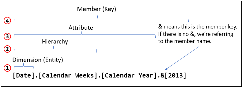
Note that while this structure is common, not all dimensions will necessarily have a hierarchy. In such cases, the dimension may directly reference attributes and members without the intermediate hierarchical level.

Sets

In the same way that calculus might be easier to understand if it’s introduced to us by its full name, “The Calculus of Change”, MDX might be easier to grasp if “sets” are referred to using its full name: Set of Tuples.

In OLAP cubes, a set is a collection of related members or tuples. A set could be defined as a selection of dimensions, grouped together for analysis. For instance, a set could contain all members of a specific hierarchy or level, or it could contain a custom-defined group of members based on a specific criteria or filter. This allows for flexible, ad hoc groupings of data, enabling users to perform targeted analyses and comparisons within their multi-dimensional data.

Note that although I say that a set is a collection of related members or tuples, in the case of members, it’s better to think of a member as a tuple of just one dimension. For example, the set {([John], [2020]), ([Paul], [2021])} is a set of tuples of the Customer and Year dimensions. Note that the set is enclosed in curly braces. The set {[John], [Paul]} could be thought of as a set of tuples of the Customer dimension, even though it looks like a set of members of the Customer dimension.

Regarding the brackets around the members, such as [John], the brackets are only necessary if the name contains something that will confuse the interpreter of the MDX. That usually means spaces and apostrophes. For example, if instead of John, the member was “John Boy”, the space between the words would be confusing to the MDX parser. So John can be simply [John] or [John], but “John Boy” must be [John Boy].

Subcubes

Subcubes are smaller, derived multi-dimensional cubes that are subsets of a larger OLAP cube. For example, your plot of land is a “subcube” of the 2D space of the surface of the Earth. They are created by selecting a range of members from one or more dimensions of the cube. Whatever falls within those ranges is the subcube. This allows for focused analysis on a particular subset of data. A subcube maintains the multi-dimensional structure of the original cube, allowing the same range of analytical operations to be performed but on a more targeted set of data.

Cellsets

Cellsets are the type of object returned by an MDX (Multidimensional Expressions) query. For most practical purposes, there might not be a noticeable difference between a cellset and a subcube.

The number of axes defined in the SELECT part of the MDX query determines the dimensionality of the resultant cellset. Essentially, a cellset is a multidimensional result of an MDX query. It appears almost indistinguishable from a subcube.

However, a key difference is that while a subcube is a defined chunk of the cube space, a cellset can be composed of multiple subcubes. The subcube represents an abstract definition of what is within the OLAP cube, whereas a cellset is the actual result returned by the query, which could encompass data from multiple subcubes.

In a sense, it’s like the difference between a shopping list for a trip to Walmart (the subcube) and the shopping cart filled with the actual items you bought, which may include items from various parts of the store (the cellset).

The cube is a multi-dimensional organization of data. When we compose an MDX, we are specifying how we want the result to look. That result are transformations taken from various subcubes within our cube.

Now that we have somewhat of an understanding of the MDX terminology, I can say that the foundational idea of an MDX query is to generate a set of tuples.

Before continuing, I need to state that for the purposes of this blog, we’re not considering how the OLAP data is physically stored, how it is retrieved, the role of aggregations, and any optimizations. We’re focused only on how we declare what is it we want to display. MDX, like SQL, is a declarative language.

Implicit Information Hidden in Plain Sight

Most nomenclatures – SQL, English, or MDX – are rife with implied information. One example that confused me for weeks in grade school was the implied symbol for carbon in a molecular structure diagram. “Oh! No element at a junction means it’s carbon!” It’s the same with MDX. I think there is so much that’s implicit that complicated MDX doesn’t sense without know the rules.

For example, the following two MDX in Figure 6 are equivalent. The first one is unnecessarily implicit about its syntax, the second is as implicit as possible.

Figure 7 shows another type of implicit syntax. The three countries (1) can be referenced without explicitly adding [Customer].[Customer Geography].[Country] because the names, Canada, United States, and France are unique in the OLAP cube. Item 2 shows the explicit reference to the three countries.

Item 3 is just a reminder that “United States” requires the brackets. Imagine if the brackets were not there–it would be hard for the query parser to tell if we intended a country named “United”, another named “States”, and forgot the comma in between.

Implicit aspects of MDX be confusing for beginners. They syntax can even seem frustratingly arbitrary. But like all “code”, it must follow strict rules, which can include cases where some text is optional.

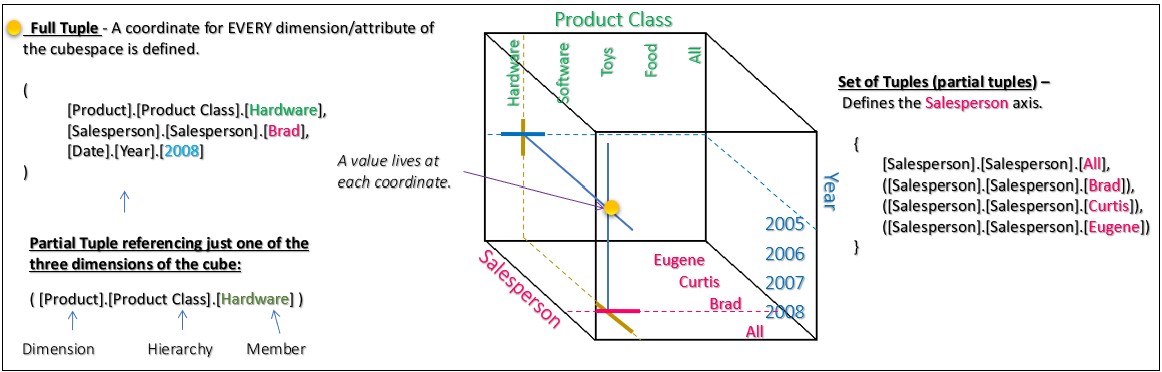
Full and Partial Tuples

A tuple in an OLAP cube is a combination of members from different dimensions that uniquely identifies a cell in the cube. This brings up what is arguably the most important concept for MDX, the notion of full or partial tuples.

1. Full Tuple: A full tuple specifies a member from every dimension in the cube. For example, if you have a cube with dimensions for Time, Product, and Location, a full tuple might look like (Time.[2019], Product.[Bikes], Location.[USA]). This full tuple precisely specifies a single cell in the cube.
2. Partial Tuple: A partial tuple doesn’t specify a member from every dimension. For instance, you might have a tuple like (Time.[2019], Product.[Bikes]). Without a location specified, this tuple can represent multiple cells in the cube.

Partial tuples can be useful for certain types of queries where you want to aggregate data across the unspecified dimensions. However, they’re less precise than full tuples, and their meaning can depend on the context in which they’re used, such as the current slice of the cube that’s being queried.

Default Members

In SQL Server Analysis Services (SSAS), the concept of a “default member” is a crucial one. A default member is the member that SSAS selects from a dimension when there’s no member specified in a certain context, often when querying multidimensional data with MDX. This plays a vital role in dealing with partial tuples in an MDX WHERE clause.

The WHERE clause is a partial tuple. The following sentence might be hard to understand. But when you do, you will be enlightened beyond the Buddha:

The elements of the WHERE clause override the default member of its respective attribute.

When you submit an MDX query with a partial tuple, SSAS will fill in the missing components of the tuple with their respective default members. This mechanism ensures that every cell in the result set corresponds to a complete tuple, thereby providing meaningful and consistent results.

The default of the default member is the “All” member. It’s automatically assigned to each attribute representing the aggregation of all members of the attribute. So each attribute can be thought of as a mini hierarchy of the [All] parent member with each member as a child.

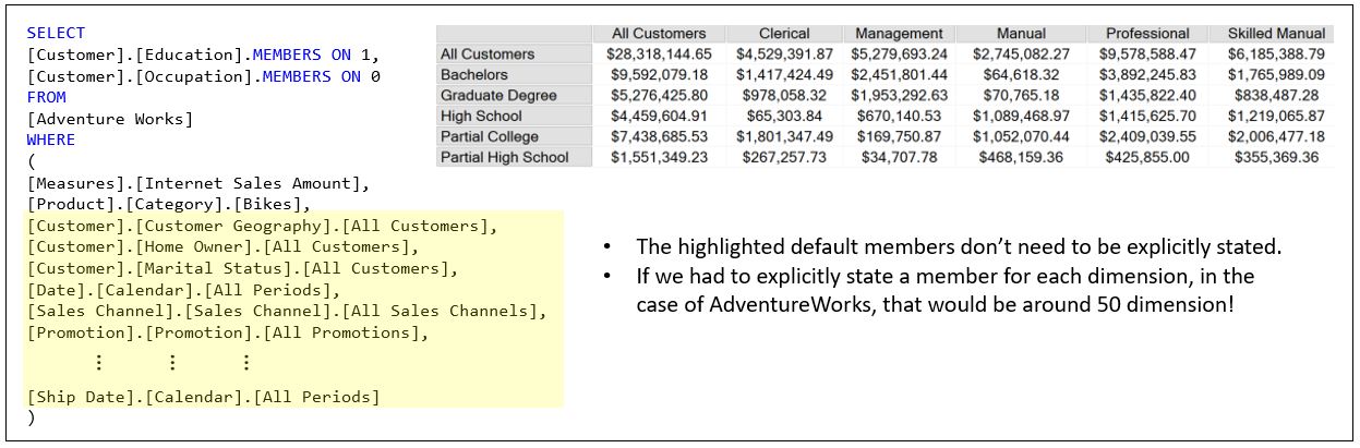
Figure 9a shows how we explicitly reference the All member. In this case, the product category all member is named [All Products].

Figure 8b shows how the [All Products] member is implicitly reference – i.e. it’s not referenced.

Note the highlighted cell in Figure 9a and 9b. Notice it’s the same. In act all of the cells have the same value. That’s because the MDX is Figures 9a and 9b are equivalent.

The takeaway is that every attribute in the cube is referenced. It’s just that most are using the implied All member.

Figure 9c shows us referencing the product category attribute again. But this time, we’re referencing the Bikes member – we are slicing to just Bikes.

We can state the difference between Figures 9b and 9c like this as: We overrode the default product category with Bikes.

Figure 9d illustrates the implicit reference to all those All members. That would be a pain to read and type if every MDX had to explicitly reference the All member!

Tuples vs Values

It can seem like a tuple and a value are kind of the same thing. For instance, consider the tuple ([Professional], [Idaho], [SalesAmount]). This tuple consists of:

• SalesAmount from the Measures dimension.
• Professional from the [Customer].[Occupation] attribute.
• Idaho from the [Customer].[State-Province] attribute.

As discussed, a tuple in MDX is a collection of members from different dimensions that together describe a specific subcube within the larger multidimensional space. Each member in a tuple is selected from a different dimension, and together they define the scope or range of data you are interested in. It’s important to note that in MDX, measures are considered a dimension as well, which can sometimes be confusing.

This tuple describes a subcube that encompasses the sales amounts for professionals in Idaho. Essentially, the tuple defines the context for the data we are querying.

While a tuple describes a subcube, a value refers to a specific data point within the cube. When we use a tuple in an MDX query, it acts as a function that returns a value. This value is the specific data point at the intersection of the dimensions and measures specified by the tuple.

In our example, the tuple ([Professional], [Idaho], [SalesAmount]) not only defines a subcube but also functions as an MDX expression that returns the sales amount for professionals in Idaho. Therefore, the value is the actual sales amount retrieved from the cube based on the criteria defined by the tuple.

Understanding that measures are dimensions too, helps clarify how tuples function in MDX. By including a measure in a tuple, we effectively specify the exact data point we want to retrieve. This approach allows us to navigate the multidimensional space of the cube efficiently and retrieve precise values.

Here’s how it works in practice:

• Defining the Subcube: The tuple defines the subcube by specifying members from different dimensions.
• Retrieving the Value: The tuple acts as a function that returns the specific value from the subcube.

Most Cubes are Sparse

OLAP cubes are generally very sparse. That means the value for most tuples is NULL – they have no value. A dense multidimensional space is one where most of the cells have a value. For that to be the case with a cube such as AdventureWorks, most salespeople would need to sell most products to each customer every day in every store.

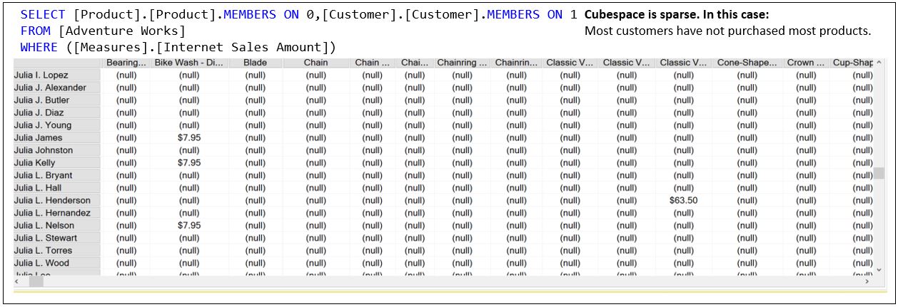
The reality is that most salespeople sell a few products to a few customers in one store every few days or weeks.

Figure 11 is an example of a 10-dimensional MDX query. How would we visualize it?

Visualizing more many dimensions (even more than 2) is a significant challenge due to the limits of human perception and the constraints of typical visualization methods which are usually two or three-dimensional. Thinking back to Figure 5, to the right of Figure 11 is some sort of depiction of what a 10D cube looks like.

In practice, tools like Power BI and Tableau handle such multi-dimensional visualizations through techniques like parallel coordinates or radar charts. Additionally, interactive features like drilling down, slicing, filtering, and rotating can help users navigate through the dimensions effectively, even if they cannot visualize all dimensions simultaneously. Advanced visualization techniques such as t-SNE or PCA might also be employed to project higher-dimensional data into lower-dimensional spaces that are easier to comprehend visually.

What Kind of Object is This?

MDX can be tricky for people who are not trained as programmers or are not familiar with the concept of functions. If you’re reading this, chances are you’re familiar with SQL and its functions or Excel functions–especially if you’re familiar with how nested functions work. In programming, a function is a named piece of code that takes inputs, performs some computation, and then gives back an output in a particular format. This notion of input and output is foundational to understanding MDX, a language designed for querying and manipulating multidimensional data.

Figure 12 shows a few examples of objects that make up an MDX:

1. Function (Query-Scoped): This query-scoped function explicitly defines a SUM operation to calculate the total Internet Sales Amount. It is scoped to this particular query, meaning the calculation is temporary and only valid within the context of this query.
2. Set – All the Occupations by a Customer: This set represents all the occupations that a customer might have. [Customer].[Occupation].[All Customers] is the member of the [Customer].[Occupation] hierarchy that represents the sum of all Occupations. “CHILDREN” is a function of the [Customer].[Occupation].[All Customers] member that returns a set of all occupations.
3. Tuple (Partial Tuple): This partial tuple restricts the [Product].[Categories] dimension to the specific category “Bikes.”
4. Results of the MDX against the AdventureWorksDW SSAS cube.

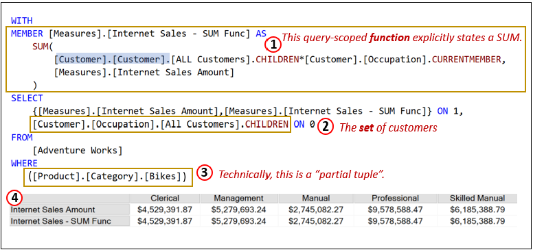
Note that for item 3, the parentheses explicitly demonstrates that the WHERE clause is a partial tuple. In this case, the parentheses aren’t necessary since there is only one element. If there were more than one, the parentheses around the entire tuple becomes necessary. For example, if we added [Customer].[Marital Status].[M], the WHERE clause would be:

([Product].[Category].[Bikes], [Customer].[Marital Status].[M])

Further, if we wanted to be as implicit as possible, we could remove unnecessary brackets:

(Product.Category.Bikes, Customer.[Marital Status].M)

Only [Marital Status] requires brackets since it has a space.

Fortunately, none of the words in this tuple example are MDX key words, otherwise they would need to remain in brackets as well. For example, if we had a dimension named “Axis”, this tuple, (Axis.[Category].[Time]), would result in an error since “Axis” is a key word.

In MDX, the “objects” you’ll work with most often are members, tuples, sets (sets of tuples), and values. Each of these is a distinct type of object, and understanding their nature – what they are, what they represent, and how they interrelate – is crucial to your understanding and effective use of MDX. Unlike SQL, where functions typically return scalar values, MDX functions can return sets, tuples, members, and scalar values.

As a review:

• A member is a point on a dimension. It represents a category of data. For instance, in a Time dimension, the members could be years, quarters, months, etc. An example MDX expression for a member might be [Time].[2023].
• Tuples, on the other hand, are combinations of members from different dimensions. They represent a specific intersection point in the multidimensional space defined by the members. For instance, ( [Time].[2023], [Product].[Laptops] ) is a tuple. This expression represents the intersection of the year 2023 and the product category Laptops.
• A set is a collection of tuples. For example, { ( [Time].[2023], [Product].[Laptops] ), ( [Time].[2023], [Product].[Desktops] ) } is a set. This expression represents the sales data for laptops and desktops in the year 2023.
• Finally, a value is the actual data that exists at an intersection of a tuple, such as sales amount or units sold. For example, [Measures].[Sales Amount] might return the sales amount value at a specific tuple intersection.

When working with MDX, it’s important to always consider the type of object a function returns. This will guide your understanding of what you can do with the result, and how to chain or nest functions together. For example, a function that returns a set, such as CrossJoin, can be used where a set is expected.

Another example, a more complicated one, is the Descendants function, which takes a member and returns a set of its descendants. For instance, Descendants([Time].[2023], [Time].[Month]) returns a set of all the months in the year 2023. The output of one function often serves as the input for another, creating a chain of computations that lead to the desired result.

Understanding and applying these concepts will enhance your mastery of MDX and allow you to leverage its full power in querying and manipulating multidimensional data.

SQL functions typically return scalar values. For example, DATEDIFF takes two dates and the desired interval and returns a number. SQL functions that return something more complex than a value usually don’t look like functions. For example, derived tables and correlated subqueries in SQL are essentially functions that take in a SQL query (with correlated subqueries taking the current row as a parameter) and return a table.

In MDX, there are multiple classes of functions based on what they return: values, sets, members, or tuples.

Towards the beginning of an MDX workshop I deliver, I warn the attendees that I will constantly ask, “What kind of object is this?” (Meaning, “And what kind of object does this function return?”) It can be annoying, but awareness of the kind of objects each piece of MDX represents is key to composing complicated MDX.

Hopefully, with this basic introduction to the objects, the understanding of the implicit nature of MDX, and the basics of how a query is resolved, that annoying question will start to pull things together.

Confusing or Overloaded Terms

Following are a few terms that I wish I clearly could differentiate when I first started with MDX.

Dimensions and Axes

I already explained that “dimension” is an over-loaded term which can mean a geometric dimension when we’re talking about multi-dimensional space or we’re talking about the OLAP object called dimension, which should really be called “Entity”.

To add to the complexity, the term “axis” also comes into play and can further complicate the understanding. In a geometric sense, an axis refers to one of the reference lines used to measure coordinates in a multi-dimensional space. For instance, in a 3D space, we have the x-axis, y-axis, and z-axis, each representing a different dimension of space.

In the context of OLAP and MDX, the term “axis” is used to describe the different perspectives or viewpoints from which data can be analyzed. An axis in MDX represents a dimension or set of dimensions along which data is organized and aggregated. For example, in a sales cube, one axis might represent time (with levels such as years, quarters, and months), while another axis might represent product categories, and yet another might represent geographic regions.

The confusion arises because both “dimension” and “axis” are used to describe ways of organizing data, but they do so in slightly different contexts and with slightly different meanings. In OLAP, “dimension” should ideally be referred to as “Entity” to better reflect its role as a categorical variable that defines a perspective for analysis. Meanwhile, “axis” in the OLAP context expresses the actual dimensions (entities) along which the data is arranged in a multi-dimensional cube.

In geometric terms, dimensions and axes are purely spatial, representing physical directions and measurements. In OLAP, dimensions and axes are abstract organizational structures used to categorize and analyze data from different perspectives.

This conflation of terms can be particularly confusing when dealing with MDX queries, where you might be specifying dimensions on different axes. Understanding the context in which each term is used and the specific nuances of their meanings in that context is crucial for clear communication and effective data analysis.

BTW, what kind of object is an axis? And what does it return? An axis is a function … so …

Granularity, Cardinality, Hierarchy Level

In OLAP, when we talk about hierarchies, a parent level is “higher” than its child. For example, Year is a higher level than Month. With that in mind, to this day, I misspeak when I say “high granularity” when I mean “low granularity”.

Concept	Example	Description
High Granularity	Day level data	Detailed, specific data
Low Granularity	Year level data	Aggregated, summarized data
High Cardinality	Employee IDs, detailed transaction IDs	Many unique values
Low Cardinality	Gender, Boolean values	Few unique values
Higher Level	Year in year, month, day hierarchy	Aggregated level
Lower Level	Day in year, month, day hierarchy	Detailed level

Balanced, Unbalanced, and Ragged Hierarchies

For some reason, my mind’s logic keeps mixing up Unbalanced and Ragged hierarchies. In my mind, I generally think they should swap names. This is probably just my problem, but I thought I’d mention it.

An “Unbalanced Hierarchy” (also known as an unbalanced tree or irregular hierarchy) is a structure where different branches of the hierarchy can have different depths. In this type of hierarchy, some branches may go deeper than others. For instance, in an organizational chart, some departments might have more levels of management than others, resulting in a hierarchy where not all paths from the root to the leaves have the same length. This uneven depth across the hierarchy can make it challenging to navigate and manage the data, as the structure is not consistent throughout.

On the other hand, a “Ragged Hierarchy” (or variable-depth hierarchy) refers to a hierarchy where some branches might miss certain levels. This is not necessarily about the overall depth, but rather about the completeness of the hierarchy at each level. For example, in a geographic hierarchy, you might have a country that is divided into states, but not all states might be divided into counties, and some counties might not be further divided into cities. This results in a “ragged” appearance because not every branch follows the same path through the levels of the hierarchy.

The reason I often mix them up is likely due to their seemingly overlapping characteristics. Both types of hierarchies deal with inconsistencies in structure, but they manifest differently. In an unbalanced hierarchy, the inconsistency is in the depth of the branches, whereas in a ragged hierarchy, the inconsistency is in the presence or absence of certain levels.

Query, Session, and Cube-scoped Calculations

In the realm of OLAP and MDX, calculations can be defined at different scopes to control their visibility and lifespan.

Query-scoped calculations are defined within the context of a single query. These calculations exist only for the duration of that specific query and are not accessible outside of it. They are useful for temporary, ad-hoc calculations needed for immediate analysis. We saw an example of a query-scoped calculation in Figure 12 (1).

Session-scoped calculations extend the visibility of calculations to the entire session. Once defined, they can be reused across multiple queries within the same user session, allowing for consistent calculation logic throughout the session without redefining it in every query.

Cube-scoped calculations, on the other hand, have the broadest scope. They are defined at the cube level and are available to all users and sessions accessing the cube. These calculations are persistent and provide standardized metrics and measures that ensure consistency and reliability in analysis across the organization. Understanding these scopes is crucial for effectively managing and optimizing the performance and usability of OLAP systems.

OLAP Cubes and Vectors

Another fascinating aspect of OLAP cubes is their relationship to vectors, which can be particularly useful in advanced data analysis techniques like clustering.

Tuples and Vectors

When we define a tuple in MDX, it typically specifies members from multiple dimensions and often includes a single measure. However, when we extend this concept to include multiple measures, we essentially create a vector.

For example, consider the tuple ([Professional], [Idaho]). If we include multiple measures, such as SalesAmount, Tax, and Freight, we get a set of tuples:

([Professional], [Idaho]) * {[SalesAmount], [Tax], [Freight]}

This yields a set of three tuples:

• ([Professional], [Idaho], [SalesAmount])
• ([Professional], [Idaho], [Tax])
• ([Professional], [Idaho], [Freight])

Each of these tuples represents a specific data point, and together, they form a vector. This vector can be represented as:

([SalesAmount], [Tax], [Freight])

Vectors in Clustering

Vectors like these can be very powerful when applying clustering algorithms such as k-means or k-nearest neighbors (KNN). By vectorizing the tuples, we can normalize the values and compare these vectors across various dimensions, such as occupations and state-provinces.

For instance, using data from AdventureWorks, we could analyze customer occupations and state-provinces. By creating vectors for each combination of occupation and state-province, we can perform clustering to identify patterns and group similar vectors together.

Practical Example

Consider the following data from AdventureWorks, focusing on customer occupation and state-province:

1. ([Engineer], [California], [5000], [400], [200])
2. ([Engineer], [Texas], [5200], [420], [210])
3. ([Teacher], [California], [4800], [380], [190])
4. ([Teacher], [Texas], [5100], [410], [205])

Each tuple here includes multiple measures (SalesAmount, Tax, Freight), forming vectors. By normalizing these vectors, we can apply k-means clustering to group similar vectors, potentially revealing insights about how different occupations and locations compare in terms of sales, tax, and freight.

Vector Normalization and Comparison

Normalization is a crucial step in this process. By scaling the values of each measure to a common range, we ensure that each dimension contributes equally to the distance calculations used in clustering algorithms. Once normalized, we can compare vectors across many occupations and states to uncover patterns and relationships.