The Ghost of OLAP Aggregations – Part 2 – Aggregation Manager

This is Part 2 of a 3-part series where I make the case that pre-aggregated OLAP is essential in this era of AI. The intent of this post is to describe just enough of how a pre-aggregated OLAP engine works for those who are unfamiliar with this technology:

1. Those who have joined the business intelligence (BI) world post-2010 when analytics was dominated by other technologies and haven’t had the opportunity to get to know OLAP cubes.
2. The BI folks who worked on OLAP cubes back in the late 1990s through about 2010 when OLAP cubes were almost synonymous with BI … and welcomed something new coming along to save them from those awful cubes.

Why would anyone care in this LLM-driven era of AI, especially after all the hype cycles of deep learning, the Cloud, machine learning and data science make it so 2000s? I explained that in Part 1—which you should read first. The main reason is OLAP cubes serve up answers to the majority of questions—including the most critical business decisions—for the majority of BI consumers from highly-curated BI data sources.

Following are sources for comprehensive understanding of the pre-aggregated OLAP products I mention in this blog (Kyvos, SSAS MD), which is beyond the scope of this blog:

• Kyvos 2025 Q3 Release documentation—Online documentation of the latest Kyvos product release at the time of writing.
• Microsoft SQL Server 2008 Analysis Services Unleashed, by Irina Gorbach, Alexander Berger, and Edward Melomed (Sams Publishing, 2008, ISBN 9780672330018). A fantastic book that covers internals.

In this post, I focus on the conceptual level of the incredibly significant work that goes into how the aggregation manager decides what to materialize, what to compute on the fly, how a “current ROLAP partition” keeps numbers fresh, and how these choices keep latency predictable for both human BI consumers and AI agents.

Much of this blog is discussion I’ve included in the hope of clarifying the value of pre-aggregated OLAP engines through comparison with other BI/AI engines. So if the next two points make sense, it’s a good indication that you can skip ahead to the walkthrough of how pre-aggregated OLAP queries use aggregations:

1. Pre-aggregated OLAP is the optimization of dimensional models consisting of additive measures which supports the ubiquitous slice and dice query pattern. The benefit is that the overall quality of the experience for the majority of questions (the ubiquitous slice and dice type of question) by knowledge workers is scalable.
2. When the volume of analytics data grows beyond what mainstream hardware can efficiently process, optimization becomes essential. That’s exactly the situation today: AI, AI agents, and IoT are accelerating data volumes, while hardware and even energy constraints make brute-force approaches unsustainable. This is what we’re facing today, so that scalability (point #1) is a critical concern.

But I still think you’ll enjoy the discussion of how BI still applies in this LLM-driven AI world of today.

Note: Although SSAS MD is still officially supported, it has long been sidelined in favor of modern, cloud-native platforms. Microsoft stopped adding new features to multidimensional years ago, focusing instead on tabular models in Azure Analysis Services and now Power BI / Microsoft Fabric. As a result, SSAS MD is no longer forward-looking—modern alternatives like Kyvos offer a more scalable, cloud-first evolution.

Background Information

For the best results from this blog, especially if you have limited or even no familiarity with OLAP cubes, please read these prior posts of this series:

1. The Ghost of MDX—Overview of subcubes and aggregations. Requisites for MDX.
2. An MDX Primer—Later, you might want to get the gist of MDX. It encapsulates the functions of analytical querying.
3. The Ghost of OLAP Aggregations – Part 1 – Pre-Aggregations—Define aggregations. If you only read one of these before tackling this blog, this is the one.

Let’s now discuss the most salient definition for this blog—MOLAP.

MOLAP, HOLAP, and ROLAP

At the heart of OLAP is a simple question: When should the computation (aggregation) happen—up front, or at query time? The answer determines whether results feel instant and predictable, or fresh but with variable responsiveness. It also drives how much load gets pushed onto the source systems versus handled by the OLAP engine itself. Really though, the answer can be “all of the above”—which is why there are the three modes of MOLAP, HOLAP, AND ROLAP.

In Part 1 I implicitly took a MOLAP view: aggregations are persisted on storage and fetched by block to the OLAP server when needed. Here, in Part 2, I’ll make that explicit and show how the Aggregation Manager decides what to pre-build (MOLAP), when to compute on demand (HOLAP/ROLAP), and how those choices keep LLM/agent tool-calls fast, governed, and reproducible.

• MOLAP: When I say “aggregation,” I mean persisted, engine-managed structures stored on durable storage (ex. cloud object storage). Think of it as a flattened, dimension-aligned copy of facts at a particular grain. It’s built offline (or on schedule) by the OLAP engine and lives on storage. At query time the engine pulls only the needed blocks from storage to an OLAP server node, where those blocks sit in memory or local disk for reuse. We don’t load the whole aggregation unless the query needs it.
• HOLAP (hybrid): If a needed aggregation doesn’t exist, the engine can fall back. It will still use persisted aggs where they exist, but for the missing slices it reads detail from the source (via the Data Source View) and computes the result on the OLAP node. This gives us fast high-level answers (from MOLAP) without pre-building every micro-grain, and it avoids processing rarely used, very low-granularity aggs.
• ROLAP (no persisted aggs): Pure ROLAP means no pre-aggregations. Every query is pushed to the source, results are computed, and the OLAP node may cache the computed result ephemerally. This is the most up-to-date path and useful for near–real-time reads, but it leans on the source system and won’t give the same predictable latency as MOLAP.

TL;DR of when to choose one of those three:

• MOLAP: Predictable latency, audited numbers, massive concurrency. Compute once, reuse everywhere.
• HOLAP: Great when users start high-level, iteratively drill down, and occasionally drill deep—build what’s hot and warm; compute the rare, low-granularity edge cases on demand.
• ROLAP: Freshest possible data, or when pre-aggregation isn’t practical (very high cardinality/volatile grains)—with the trade-off of variable latency and higher source load.

Other Terms

These other terms are good to know for this blog. They are entries in the glossary: Aggregation Design, Root aggregation, On-the-fly aggregation, slice and dice query pattern.

Shiny Things

Here is a curiosity that’s worth exploring—because it’s an example of a bigger lesson. That is, older things aren’t necessarily superseded by shiny new things. Often, it’s more that the shiny new things are a gift to short attention spans. Whatever the new thing is good at becomes the reason why the old thing wasn’t the magical answer to everything, and thus we can throw all that old stuff away and work on this new magical technology.

With that in mind, OLAP and LLMs have some things in common. SQL Server Analysis Services (SSAS MD), the dominant OLAP before 2010, came out with as much promise for BI as LLMs did for AI with ChatGPT 3.5 in November 2022.

Some commonality is that both OLAP cubes and LLMs are highly-processed structures computed from massive amount of messy, heterogeneous data which then is compiled into an intermediate form that people and systems naturally relate to. OLAP cubes compile numbers into a dimensional, pre-aggregated index; LLMs compile text/code into a semantic index encoded in parameters. In both cases, we pay compute up front so downstream use is faster, and we extend at runtime when the core isn’t enough (HOLAP/ROLAP for cubes; retrieval/tools for LLMs).

Both the old SSAS MD and today’s LLMs failed in their respective hype cycles. SSAS MD never became the almighty “Universal Dimensional Model” (UDM) of BI, and LLMs seem to be reaching diminishing returns, falling short of AGI on their own. But that’s because both are only components within larger systems. OLAP cubes are the optimized, customer-facing layer of highly curated analytics platforms. LLMs are more like the mechanism that turns our fleeting thoughts into language, and language we hear back into patterns of meaning within the web of neurons.

The point is, OLAP didn’t become obsolete. It faded into the background, but it didn’t disappear. The same is true across the broader history of AI: Prolog/Lisp in the 1980s (expert systems and reasoning), the Semantic Web in the 2000s (knowledge graphs of linked data and ontologies), Deep Learning in the 2010s, and now LLMs in the 2020s (language modeling and generative AI). Each had its moment of hype, fell short of replacing everything, and ultimately settled in as a vital building block—see my series, Prolog in the LLM Era and Enterprise Intelligence for how Prolog and Knowledge Graphs, respectively, still have a place in the AI world.

In the same way, LLMs are a fundamental component of AGI—but only one piece. Much more remains to be developed, some of which I hint at in other blogs on this site. This is no different from thinking the neocortex alone is responsible for human intelligence, nor are LLMs alone the key to AGI/ASI.

The subject this post, Part 2 of the series, is a highly-responsive, highly-trusted data source for AI to access—OLAP as the customer-facing layer of BI. I’ve written other blogs detailing the justification for OLAP in this LLM-driven era of AI:

• TL;DR – Pre-Aggregated OLAP in the AI and IoT World—LLMs facilitate questions that are bigger and more complex, while pre-aggregated OLAP makes answers cheap, governed, and fast. Use cubes as the front door; let agents handle mapping, orchestration, and fallbacks to HOLAP/ROLAP when a query genuinely needs the live leaf.
• All Roads Lead to OLAP Cubes – Eventually—The moral of all roads lead to OLAP isn’t that aggregations increase performance. The moral is that it’s tough to manage them. If you read only one on this list, this is the best choice.
• The Role of OLAP Cube Concurrency Performance in the AI Era—I offer that AI (LLMs, agent workflows) multiplies BI query volume, so concurrency—not just single-query speed—becomes the bottleneck. Pre-aggregated OLAP cuts data reads/compute, enabling sub-second responses at high parallelism and supporting AI builds like knowledge graphs/strategy maps.
• The Role of OLAP Cubes in “Enterprise Intelligence”—Places BI/OLAP as a core facilitator of an Enterprise Knowledge Graph architecture—delivering speed, scale/concurrency, and powering ISG/TCW structures—while treating pre-aggregations as a resource-preserving cache that bridges structured and unstructured/LLM-enriched analytics in the AI era.
• 4 Ways in which Smart OLAP™ Serves the Data Science Process—Shows how cubes help data science end-to-end: as a fast, curated EDA source; as quick ad-hoc cubes to align teams; as production support for model monitoring; and by materializing ML outputs (scores/clusters) into a “Property” dimension for business slicing.

Aggregation Manager

If you read, All Roads Lead to OLAP Cubes – Eventually, you saw that the management of an aggregation design is the most important job of a MOLAP product (SSAS MD, Kyvos). Of course, the reason we need to manage the aggregation design is because we can’t materialize every combination of attributes.

A typical enterprise cube has about 10 to 25 dimensions and, across them, hundreds of attributes and levels (two hundred to a thousand is common). Only a portion are worth aggregating (because users will slice and dice by them), but even that short list creates far more combinations than we can ever build.

For example, if you have a short list of, say, 20 attributes that people actually slice by, the number of possible groupings is already around one million. At 30 attributes it’s about one billion. At 50 attributes it’s roughly a quadrillion.

Even modest choices multiply quickly. For example: eight dimensions, each with three useful levels—about 6,500 combinations. If some dimensions have five or six levels, the total jumps much higher, fast.

Treat pre-aggregations like a portfolio: fixed storage and build time invested only where they measurably reduce latency on real workloads. Everything else stays lean and is served from the root with smart partitions.

Because of this, aggregation design is akin to a sophisticated budgeting and allocation exercise: balance size and build time against how much time the pre-agg actually saves on real queries compared to rolling up from the base fact table (the “root aggregate” path).

For any candidate pre-aggregation, we must consider:

• How big will it be? Estimate rows by multiplying the distinct values of the grouping attributes. More distinct values means more rows and more storage. Low-level aggregations, for example 10 million customers who have an average of 100 invoices, is quite large and goes against the typical drill-down pattern of OLAP.
• How long will it take to build and refresh? Think in wall-clock time during your load window.
• Who will it help, how often, and by how much? Look at actual workload: which query shapes are common and painful. Keep what meaningfully cuts their runtime.

Keep a candidate only if the time saved on real queries clearly outweighs the storage and build cost over the period you care about.

In SSAS MD, there was something called the “one-third rule”. By default, SSAS MD wouldn’t include an aggregation if the number of rows exceeded one third that of the fact table.

The constraint settings for the Aggregation Manager:

1. Storage ceiling. For example: “Pre-aggregations can consume at most 20–30% of the compressed size of the base fact.”
2. Processing window. For example: “Nightly builds finish within two hours; incrementals within 15 minutes.”
3. Targeted benefit. For example: “Focus on the top 20 query shapes by frequency times pain.”
4. Cardinality guardrails. Skip any grouping whose estimated row count approaches a large fraction of the base fact; those rarely pay back.
5. Diminishing returns rule. After you’ve covered the hot spots, raise the bar for adding more.

Aggregation Design Wizard

In OLAP, an aggregation design is the plan that decides which pre-calculated summaries (aggregations) should be built and stored so queries can be answered quickly. At the leaf level (root aggregation), a cube is roughly as large as the underlying fact table—essentially a flattened view. True aggregations sit above that leaf: small, pre-computed results that can be reused by many queries. The design challenge is to balance storage and processing cost against query speed, since building all possible aggregations (the full lattice) is impractical.

• SSAS MD’s Aggregation Design Wizard tackles this by picking a set of summaries per partition, trading storage and build time for faster query performance. By default, its algorithm assumes all queries are equally likely; designers then refine the design, historically using usage-based optimization driven by query logs.
• Kyvos’s equivalent is its Smart Aggregations layer, which plays the same role but is ML-driven and continuous. Instead of static designs per partition, Kyvos monitors actual query patterns and the shape of the data to decide which aggregates to add, drop, or refresh. It supports incremental updates as new data lands, keeping cubes responsive without full rebuilds.

Both systems boil down to the same principle: managing a cache of summaries. SSAS exposes this explicitly as aggregation designs (one per partition) that BI developers tune. Kyvos automates it, using usage-aware algorithms so you “build once, reuse everywhere” and adapt automatically as workloads change.

Kyvos vs Databricks and Kyvos vs Snowflake

A common question I get is: Why do we need Kyvos when we have Databricks or Snowflake? A common misunderstanding I run into with customers is based on not knowing how Kyvos differs from Databricks or Snowflake. Of course, in the enterprise BI/analytics world the battle of data platforms is very often between Databricks and Snowflake and their differences are relatively more well discussed and understood.

My intent is not to throw Kyvos into that mix as a contender. Rather, I intend to make the case that all three serve distinct purposes, that in concert can create a more robust system of expert platforms. In other words, let each do what it does best, independently of each other, working together in a loosely-coupled fashion.

To help express the value of MOLAP in such a hybrid system, I need to contrast it with these other approaches. This blog isn’t a bake-off of analytics data platforms. Over the past few years all of the products have evolved, with tentacles reaching away towards the core capabilities of all the others. But they still excel at their respective origins:

• Databricks for scale-out, low-level, iterative data processing, usually into machine learning models,
• Snowflake as a truly scale-out data warehouse.
• Kyvos as the Cloud-scale optimization of dimensional modeling and naturally a semantic layer. Pre-agg OLAP traces its history as a semantic layer back to 2005 when SSAS MD positioned itself as the Unified Dimensional Model (UDM).

The difference between Databricks and Snowflake starts with where they attack analytics. Databricks approaches from the data science side, while Snowflake comes from the BI analyst side. However:

• Databricks’ Lakehouse narrows the gap by layering Delta Lake over Parquet files, adding ACID transactions, CRUD operations, schema enforcement, and time travel. These features let a raw data lake behave much more like a governed warehouse, enabling the creation of reliable, structured tables on top of cloud object storage.
• Snowflake has edged toward Databricks’ domain, extending beyond classic BI workloads. Support for semi-structured and unstructured data, data pipelines, and even data engineering tasks shows Snowflake leaning into workloads that once belonged firmly to data lake platforms.

In short, each platform has stretched toward the other’s strengths—yet both remain anchored in their origins: Databricks in large-scale, iterative data processing, and Snowflake in enterprise BI and warehousing.

Data science calculations are often a completely different animal from BI formulas primarily consisting additive aggregations. As opposed to formulas where we plug in values, they’re more intricate, often require access to case-level detail and algorithmic thus they’re highly iterative. Data scientists need the freedom to try out different ways of condensing and reshaping data from its most elemental, lowest-granularity form.

In contrast, OLAP is built to optimize the kinds of questions most knowledge workers ask: sums, counts, and averages. That’s the bread-and-butter of business analysis, and OLAP makes those queries fly. The Lakehouse is trying to straddle both: flexible enough for data science, but familiar enough for BI.

Like everything else, MOLAP cubes aren’t the answer to everything related to BI and analytics. Similarly, relational databases such as SQL Server and Oracle weren’t the best answer to everything data—as the NoSQL rebellion of the 2010s demonstrated. New engines appeared because different problems needed different shapes. What MOLAP does is optimize the storage and retrieval of data required for slice and dice queries.

Why Did SSAS MD Move to the Backburner?

Around 2010-ish it looked like SSAS MD would be eclipsed—ironically by its own sibling, SSAS Tabular (which became Azure Analysis Services). Tabular ran in-memory, stripped away a lot of MD’s aggregation/memory plumbing, consequently configuration complexity, and replaced MDX with DAX, which felt closer to Excel for most people.

SSAS Tabular didn’t replace SSAS MD—it right-sized a big chunk of workloads. By 2010, servers with 64GB+ RAM were normal in enterprises, and compression (VertiPaq) meant many models were an order of magnitude smaller in memory. Most business models actually fit, so Tabular delivered great interactivity with a simpler mental model.

But the edge cases never went away. Some SSAS MD cubes were—and still are—too large or too granular for in-memory only. Tabular also lacked several “advanced” SSAS MD features early on (it was a V1 advanced from some advanced Excel Add-ins), and being in-memory meant reloads on service start. Those realities kept MOLAP-style pre-aggregation relevant, especially for very high cardinality, very wide models, and heavy concurrency. There’s always a place for an option that is scalable to beyond a couple standard deviation from the average.

In parallel, the scale-out story matured on two fronts:

• MPP data warehouses: PDW which became Synapse, Redshift, and Snowflake—although Snowflake is more than MPP. They gave us distributed SQL over detail—the governed system of record for joins, windows, and exact reporting. Snowflake in particular is cloud-native in the way Kyvos is a cloud-native take on MD: both rethought their predecessors for elasticity and cloud storage.
• Spark/Databricks became the compute fabric for machine learning and data science—massively parallel transforms, feature engineering, and training. Spark is not a data warehouse; it’s where you reprocess low-granularity data many times while you sweep features and hyper-parameters.

From early on (SQL Server 2000), SSAS MD brought ML to the cube (data mining algorithms over cubes or source via DSV). But it was ahead of its time; “data mining” was fringe in many orgs then, so adoption was limited—not because the idea was wrong, but because the culture and tooling around it wasn’t ready within general enterprise domains.

What that history means now (even in this era of LLM-driven AI):

• Pre-aggregated OLAP (MD lineage, Kyvos in the cloud) is still the front door for governed facts: conformed dimensions, curated measures, role security, lineage, predictable latency, and compute-once/read-many for the sums, counts, rates, and ratios that still dominate decision-making. With more consumers (knowledge workers + AI agents), pre-aggs prevent a storm of redundant scans.
• Tabular/in-memory is great when the entire model fits in memory and you want rapid interactivity with simpler semantics. It’s not the right hammer for extreme cardinality or petabyte-scale detail.
• Cloud MPP DW is the source of truth at leaf level—detailed reporting, exact SQL, window functions, and any feature engineering that truly needs transactions/cases.
• Spark/Databricks is the “reprocessing engine”—iterate over low-granularity datasets, build pipelines, train models, and sweep feature combinations and hyper-parameters at scale.
• Data lake is the catch-all for wide/heterogeneous inputs (logs, telemetry, external drops, embeddings) you’ll join to DW/cubes when they prove their value.

Put simply:

• Ask an OLAP cube when the question is additive slice-and-dice (and you need speed, governance, and concurrency).
• Ask the DW when you need exact detail.
• Ask Spark when you need to redo the same heavy work many times.
• Keep the lake for everything messy you’ll harvest into the other three.

Letting Each Engine Do What They Do Best

Let’s look at how Kyvos, Snowflake, and Databricks might play well in a system where each plays to its strength. Again, I’m a big fan of all three. To review:

• Kyvos is the pre-aggregation specialist. Its Smart OLAP cubes are built precisely for high-concurrency business use—scales out for very many users, human and AI. It knows how to manage which aggregations to build, how to store them efficiently, and how to deliver consistent, governed numbers every time. That’s the semantic backbone of the system: business users always see the same definitions and the same answers.
• Snowflake attacks analytics from the BI side. It looks like a classic data warehouse of tables. But unlike a true RBMS like SQL Server which are designed for OLTP query patterns, it’s designed for OLAP query patterns. Snowflake’s query mechanism is smart enough to automatically recognize when a materialized view can be useful in a query. Its semantic views allow logical definitions of metrics and dimensions that multiple tools can share. It’s not as deep as Kyvos in semantic governance, and not as raw in computational power as Databricks, but it provides a broad, reliable middle ground for BI workloads.
• Databricks attacks analytics from the data-science side. Spark is general-purpose, high-power compute—well beyond slice-and-dice—able to run algorithms in Scala/Python/SQL at scale for highly iterative, complex workloads on case-level detail. In Databricks’ medallion pattern, “Gold” means consumption-ready data (often aggregated, sometimes just curated/denormalized)—it’s not a cube. Unity Catalog supplies governance and lineage, and Metric Views in UC centralize KPI definitions, but they’re semantic objects, not a pre-aggregation store. You can speed hotspots with materialized views, caching, and Photon, yet Databricks does not include a Kyvos-style multidimensional pre-aggregation manager that designs/maintains a lattice and routes queries for high-concurrency slice-and-dice. In practice, Databricks complements a cube engine rather than replacing one for governed, interactive BI at scale.

Each of these, with growing lists of features that extend their reach beyond its core, can serve the customer on its own. But the stronger view is to treat them as parts of a best-of-breed system:

• Kyvos as the semantic layer and pre-aggregation engine.
• Snowflake as the flexible (not constrained to dimensional models) BI warehouse with materialized views and logical models.
• Databricks as the heavy compute engine for data science.

Together, they create an ecosystem where business reporting, ad hoc analysis, and advanced data science all have a place, each workload being executed where it fits best.

Figure 1 illustrates where MOLAP cubes still fit in the modern analytics stack—here from the point of view of a data scientist, a non-traditional MOLAP consumer. This diagram shows how a data scientist can use three complementary data sources—an MPP cloud data warehouse, an OLAP cube, and its primary axe, Databricks/Spark cluster. As mentioned above, please read, 4 Ways in which Smart OLAP™ Serves the Data Science Process, for more details.

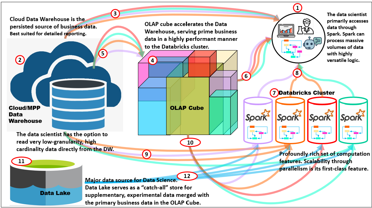
Here are descriptions of the numbered items of Figure 1:

1. Data scientist and AI Agents: Most exploratory and training work originates in Spark notebooks. Spark (8) lets us reprocess low-granularity data repeatedly while we vary features, parameters, and hyper-parameters.
2. Cloud MPP Data Warehouse (persisted truth): The DW is the governed system of record, best for detailed reporting, SQL joins, and exact numbers. When the data scientist needs data at the most granular level (which could be very many rows), read it from here. Examples: Azure Synapse, AWS Redshift, Snowflake.
3. Cloud MPP→Data Scientists: The cube materializes business-ready aggregates over conformed dimensions. It answers most additive slice-and-dice questions with predictable latency and serves as a reliable feature source for many models (counts, sums, rates, quantiles/sketches, transition counts).
4. OLAP cube: The most important data in the enterprise is locked and loaded for high performance analytical activities.
5. DW→Cube feed: Dimensions and facts flow from the DW into the cube’s root and designed aggregations, keeping semantics aligned and numbers auditable.
6. Cube→Spark: For ML, pull pre-aggregated features directly from the cube (ex. customer-30-day totals, store-week rates). This avoids recomputing the same aggregates in Spark and keeps governance intact.
7. Databricks cluster (compute fabric): Spark provides the first-class parallelism to reshape large datasets, engineer features, train at scale, and run grid/Random/Hyperopt searches.
8. Spark→Data Scientists: Use Spark when you must reprocess the same low-granularity data many times (feature sweeps, hyper-parameter tuning, cross-validation), or when logic is more algorithmic than declarative SQL.
9. DW→Spark (leaf access): When features require true transaction/case rows (ex. price dispersion, basket co-occurrence, sequence timing), read the detailed DW tables directly.
10. Cube as feature store (compute-once, read-many): For stable, additive features, let the cube be the compute-once layer. It reduces redundant processing across many experiments and agents.
11. Data lake (catch-all): The lake stores raw/semi-structured data—logs, telemetry, images, external drops—that don’t fit neatly in the DW yet but are valuable for ML.
12. Data Lake→Spark: Enrich cube-based business features with lake data in Spark (ex. telemetry joins, embeddings). Promote proven features back to governed layers.

An interesting thought is that Databricks can act as part of the ETL/ELT compute fabric that creates enriched fact tables and dimensions—not just domain extracts but heavy transforms and ML-derived outputs (forecasts, propensities, clusters, anomaly scores). These curated tables land in the Cloud DW and then surface in the OLAP cube as sliceable measures or attributes, keeping governance while avoiding repeated recompute. For example, recommendation affinity scores , causal uplift/experiment effects by cohort, time-to-event estimates such as expected churn date. I outline this pattern in 4 Ways in Which Smart OLAP Serves the Data Science Process.

TL;DR of when to choose which:

• OLAP cube: curated, additive features and KPIs; fast, governed, high concurrency; ideal for compute-once, read-many and for agent tool-calls that need deterministic facts.
• Cloud/MPP DW: exact, leaf-level queries; heavy joins/windows; detailed reporting.
• Databricks/Spark: iterative reprocessing at low granularity; feature pipelines; model training and hyper-parameter sweeps.
• Data lake: broad, heterogeneous sources; experimental or external data you’ll join to DW/cube later.

Table 1 compares the three products broken down by the primary capabilities of MOLAP cubes.

Feature / Attribute	Kyvos	Databricks	Snowflake
Pre-Aggregation	True MOLAP engine (Smart OLAP™). Builds cubes with extensive pre-aggregations for predictable latency and concurrency at scale. Supports incremental cube processing so only changed/new data is processed, reducing overhead.	Materialized views provide MOLAP-like benefits but without multidimensional cube structures. They must be explicitly defined, stored in Unity Catalog, and refreshed on schedule or manually.	Materialized views are robust, automatically refreshed, and automatically recognized by queries. Not cube-like, limited in number, and not auto-managed for coverage.
Query Process	Specialized OLAP engine optimized for hierarchical drill-down/up/through. Queries are resolved via pre-computed aggregates; predictable under heavy concurrency.	Distributed Spark engine with massively parallel compute. Handles highly complex, iterative, case-level queries—far more general-purpose and flexible than OLAP engines.	SQL engine with strong pruning, clustering, and cost-based optimization. Excellent for BI workloads and moderately complex analytics, though less versatile than Spark.
Aggregation Manager	Automated cube design & AI-assisted optimization (decides which aggregates to pre-build and how to balance storage vs. query speed).	No explicit aggregation manager. Materialized views must be defined and managed manually or through pipelines; Unity Catalog governs them but does not optimize placement or selection.	Optimizer recognizes when a materialized view can be used automatically, but choosing which to build/retain is manual. No higher-level aggregation design assistant.
Semantic Layer	Full semantic layer. Centralized and governed definitions for measures/dimensions. Consistent across BI tools with business logic abstraction built-in.	Unity Catalog provides governance, metadata, lineage, and access control. It is not a full semantic layer—business metrics and logic consistency must be defined elsewhere.	Semantic Views allow logical modeling of metrics and dimensions across queries. Useful for consistency but lighter than Kyvos’s governed semantic layer.

As a reminder, my intent for this comparison isn’t as a “bake off”, to shine any of these products in a better light than the others. I think they are the best of breed in relation to their core capabilities—which is why I use these products as “icons” of their respective core capabilities. All three can technically stand alone as an analytics platform with varying degrees of capability on a variety of features, but as a system of platforms, each filling different core capabilities, it creates something much better.

Please keep in mind that for simplicity I haven’t included equally important databases filling other specialties of a system of platforms for analytics:

• Graph DBs (Neo4j, GraphDB): For scale-out Knowledge Graphs (database for entities, ontological relationships, lineage, policy, and reasoning), particularly the Enterprise Knowledge Graph (EKG), the main protagonist of my book, Enterprise Intelligence.
• Vector stores (Pinecone): Specializes in questions that measure the similarity between text sections, as well as for RAG queries, retrieval-augmented reasoning, deduping synonomous phrases, and semantic joins.
• Open-schema document stores (MongoDB, CosmosDB): Fast landing zones for semi-structured content, prompts/completions, tool traces, and app configs. For CosmosDB, it also is a fantastic landing zone for event-driven architectures:
  • CosmosDB integrates natively with Azure Event Grid and Change Feed, which make it an excellent foundation for event-driven architectures. Every insert/update/delete operation can be streamed as an event to downstream services, without polling. That makes CosmosDB not just a landing zone, but a trigger point in a reactive system. It’s a natural fit for scenarios where semi-structured data (like IoT events, user activity, or tool traces) needs to fan out to analytics pipelines, queues, or ML services.
  • MongoDB also supports event-driven patterns, primarily through Change Streams. These streams let applications subscribe to data changes (at collection, database, or cluster scope) and react in near real-time. It’s not as tightly woven into a cloud-native event fabric as CosmosDB is with Azure, but functionally, it enables the same paradigm: changes in the document store can drive workflows, analytics updates, or notifications.

Speaking of events (MongoDB, CosmosDB), I’d like to throw out the “Time Solution” I describe in my book, Time Molecules (June 4, 2025). I refer to it as the event-centric side of OLAP.

Cloud Storage Foundations Across Platforms

All three analytics platforms shown in Figure 1—OLAP Cubes, Data Warehouse, and Spark—share a core dependency: they persist data on highly scalable cloud storage. Each platform applies its own storage architecture and optimizations to make that storage performant and manageable.

• Databricks – Delta Lake: Databricks builds on open-format data lakes using Delta Lake, an open-source storage layer. It adds ACID transactions, schema enforcement, and time travel to Parquet-based storage via a transaction log, making the raw lake behave much more like a governed warehouse while preserving flexibility and scale.
• Snowflake – Micro‑Partitions: Snowflake ingests data into its proprietary storage, organized as micro-partitions. Each micro-partition is automatically compressed and accompanied by metadata that drives efficient query pruning and clustering. This approach ensures strong query performance and elasticity—albeit within Snowflake’s proprietary format.
• Kyvos – Proprietary Cube Storage: Kyvos employs its own cube storage format, extensively optimized for high-performance OLAP. Data is pre-aggregated into cubes—partitioned and indexed for rapid drill-down queries in large, high-cardinality datasets. This specialized structure underpins Kyvos’s Smart OLAP™ engine.

OLAP Cube Alternatives to Classic Pre-aggregated cubes

Lastly, it makes sense to compare the benefits of MOLAP cubes against non-persisted OLAP engines. Again, there are legitimate tradeoffs that mean they are more or less valuable under different circumstances.

• On-the-fly aggregates (semantic layer / “autonomous” aggregates): Platforms like AtScale create and manage aggregate tables as queries arrive, warming a cache around the parts of the model users actually hit. As patterns repeat, the engine predicts/creates aggregates and rewrites queries to them; performance improves the more workloads concentrate on “hot” slices. Think of it as dynamic, workload-driven pre-aggregation. The result is that first-time queries are “cold” (slower), and if many knowledge workers roam widely across the cube space, the engine may churn aggregates or hit storage/compute budgets more often. You still set guardrails (eviction, caps) to avoid runaway cache growth.
• “On-the-fly” via Tabular/AAS storage modes + aggregations: In the Microsoft stack, Tabular/Power BI models mix Import (in-memory) and DirectQuery (passthrough) with an Aggregations feature. Hot summaries live in-memory; cold or fine-grain slices route to the source. It’s functionally similar to on-demand pre-aggregation with rule-based routing. The result is that cold paths depend on source speed; the modeler must choose grain and storage modes wisely (Dual/Import for common groups, DirectQuery for long tail).

BI and the LLM-driven Era of AI

It’s easy to forget that BI, machine learning, and AI were at one time very fringe. Long before “data scientist” was a common title, a handful of high-end teams at niche enterprises (ex. hedge funds, enterprises researching advanced technologies, intelligence agencies) were already doing modeling and advanced analytics—custom stacks, niche tools, and heavy engineering. For BI, while most organizations lived in Excel, a minority invested in data warehousing and OLAP starting in the early 1990s (the Inmon and Kimball era), data warehouses for historic, reliable, integrated reporting generated with relative ease.

AI followed a sort of similar curve. It jumped from research labs to the enterprise mainstream faster than BI (after all, everything is faster in the AI realm)—and in parallel it hit the general public via consumer chat apps. Those are not the same audience. Enterprise adoption still has to satisfy governance, lineage, security, SLAs, and cost controls.

When analytics moves from bleeding edge research assigned to elite teams to broad enterprise use—and now to AI agents as first-class data consumers—pre-aggregated OLAP becomes more, not less, important. It’s the mechanism that turns raw detail into governed, repeatable, low-latency facts that can be safely reused by thousands of people and tools. BI data is an AI’s “sense” of an enterprise’s recent experience. Existing BI as the spearhead for the adoption of AI in the enterprise, is really the storyline of my book, Enterprise Intelligence.

The analogy stops where cube results are deterministic and auditable—same slice, same number, with lineage and cell-level security. LLM outputs are probabilistic and must be grounded against governed data. ROLAP/HOLAP joins trusted sources at query time; RAG fetches unstructured content that still needs validation. Treat them as complementary: cubes supply facts, while LLM makes sense of complex information and RAG orchestrate, explain, and route.

Pre-Aggregated OLAP as the Semantic Layer of Highly-Curated Data

LLMs do hallucinate. And as I write this, LLMs are very useful if I need answers based on well-known information. But if I try to express anything that isn’t well-trodden, LLM help is more trouble than it’s worth. With that said, the notion of pairing LLMs into a symbiotic relationship with the SME-authored (or SME-supervised) knowledge graphs is growing. Additionally, existing BI platforms offer another highly-curated data source geared towards serving up analytics-focused information.

Data Mesh Accelerating the Onboarding of Domains into the BI System

We also moved past the “one giant cube.” In a data-mesh style, we build domain cubes and connect them with mapping tables. It’s routing across governed datasets, not a single monolith. And like LLM adapters, cubes can be adapted without rebuilding via calculated measures, named sets, and perspectives—semantics layered on top of pre-aggregations. I discuss this further in my blog, Data Mesh Architecture and Kyvos as the Data Product Layer.

Thie successful acceleration of the onboarding of more domains means many more BI consumers—knowledge workers, execs, finance, data scientists—and now AI agents that help map, route, and guard access across domains. Pre-aggregated cubes remain the safest, fastest way to serve them all.

Cubes are the best choice as the customer-facing layer because:

• Speed at scale. Pre-aggregations turn warehouse scans into block reads. With thousands of humans and agents, “compute-once, read-many” keeps latency predictable.
• Determinism & governance. Cubes are curated: conformed dimensions, cleansed measures, role-based security, lineage. Agents need hard ground truth they can’t accidentally mutate.
• Concurrency economics. Agents amplify traffic. Pre-aggs prevent redundant work and protect upstream systems from stampedes.
• Semantic alignment. Conformed dims plus mapping tables let agents stitch Sales↔SCM↔Finance without semantic drift.
• Freshness without fragility. MOLAP where it pays; HOLAP/ROLAP partitions for slices that must be current. (SSAS solved this years ago; modern engines keep the pattern.)
• Additive reality. Most operational questions are still sums, counts, rates, and simple ratios over slices. Cubes answer those instantly and reproducibly.
• Agent-safe by design. Tool calls hit secured cells; agents can propose mappings, spot odd access patterns, and hand off only what a role allows.

The AI-Accentuated BI Layout

BI data is highly curated data, thus highly-trusted. The BI stack builds a secure layer where data is cleaned, governed, and structured into cubes or models that business users can rely on. That same foundation now opens the door for AI agents—not as replacements, but as embedded assistants that can be deployed at many points across the BI landscape.

Figure 2 shows how agents can be woven directly into the BI ecosystem. Each icon marks a place where AI can add value: attached to data products as gatekeepers, embedded in visualization tools as copilots, working with managers and executives as personal assistants, or helping stewards maintain mappings across domains. The power comes from the highly-curated BI data layer: because the data is already secured, conformed, and trusted, agents can operate with confidence, delivering assistance without eroding governance.

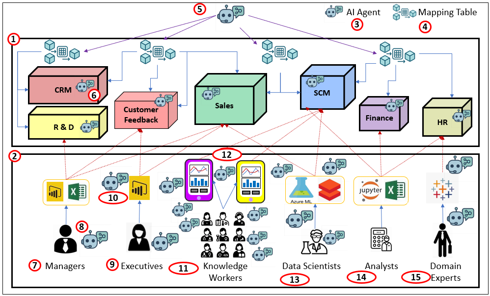
Following is a guided walk through each part of the diagram. From domain OLAP cubes that act as data products, to BI consumers, to the specialized roles of analysts, executives, and scientists, you’ll see how AI agents can be integrated throughout the BI world—always grounded in the governed BI layer.

1. Domain OLAP Cubes (Data Products) Conformed, user-friendly, and highly curated. Pre-aggregated for high performance with intuitive security (row/column, subcube, down to cell). Each cube is a data product in a mesh.
2. BI Consumers & Interfaces All the front ends people actually use—dashboards, Excel, notebooks, custom apps.
3. AI Agent Icon The assistant symbol used wherever agents participate.
4. Mapping Table The crosswalk that links dimensions/measures across domains.
5. AI-Assisted Mapping Agents suggest and validate matches, flag conflicts, and help stewards and SMEs maintain the mappings.
6. Cube-Scoped AI Gatekeeper An agent attached to each cube/data product: understands schema and policies, enforces access, capable of encoding a query from the prompt it receives, including schema information.
7. Managers Traditional BI consumers—tactical decisions, operational KPIs.
8. Personal BI Copilot Agent embedded with the consumer: fetch, explain, warn, and propose next steps.
9. Executives Strategic consumers—may not click through daily, but initiate BI work and consume curated views.
10. Visualization Copilot Agent inside the viz tool (think Copilot in VS Code): build charts, fix queries, narrate results.
11. Knowledge Workers Everyone with a job to think. Mobile-first, embedded BI in everyday tools; broadest audience.
12. Mobile Apps Targeted, quick-to-build apps tailored to roles and tasks.
13. Data Scientists Not classic BI users, but benefit from cube features; escalate to leaf data when needed.
14. Analysts Cross-domain explorers—strong business context and analytic skills; less ML-heavy than data scientists.
15. Domain Experts Deep in a single area; in a mesh, often the primary consumers of that domain’s data product.

Yes, that was a lot of ado before we got to the actual topic of this blog—enough background to show how pre-aggregated OLAP acts as an aggregation manager. But we had to explore why this is still important. So, without further ado, here it is …

How an OLAP Query Is Processed

Every OLAP query is, at its core, a hunt for the fastest valid path to an answer. The engine doesn’t just scan a table—it decomposes the request, checks what’s already been computed, and decides whether to serve from cache, from persisted aggregations, or to calculate on the fly. This hierarchy of options is what makes OLAP predictable at scale: you don’t always hit the raw warehouse; instead, you often get a pre-built summary that was designed to be reused.

Figure 3 shows the flow. The data warehouse remains the system of record, over which a dimensional model is painted. From that model, a MOLAP cube is built with two main layers: the root aggregation (the lowest-grain fact flattened at dimension keys) and a set of designed aggregations chosen for reuse. Hierarchies provide the paths for roll-ups. At query time, the OLAP server decomposes the request into subcubes, looks for persisted matches, and, if necessary, falls back to root-level or ROLAP-style reads from the source. Along the way, it caches what’s hot and logs what’s missing so the aggregation manager knows what to build next.

The result is a system that blends speed, efficiency, and freshness: persisted hits for deterministic performance, roll-ups from root when needed, and live warehouse reads to ensure the newest data is always available.

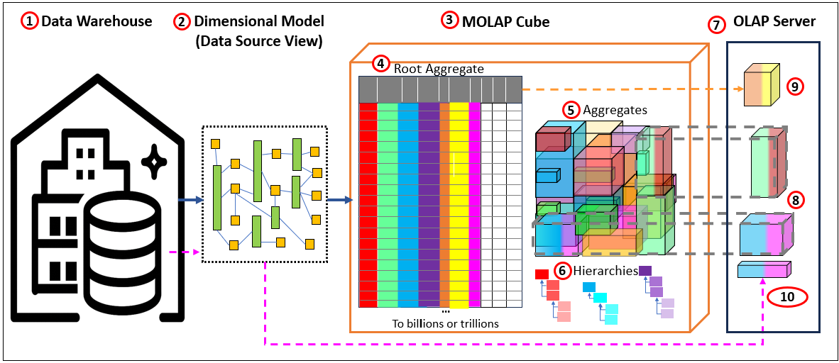
Here are the descriptions for Figure 3:

1. Data Warehouse. The primary data source of the OLAP cube. The layout is usually similar to that of a regular (3rd Normal Form) relational database. Or it can be in the form of a dimensional model.
2. Dimensional Model. The warehouse is the system of record. It doesn’t have to be a physical star; the dimensional model paints a virtual star/snowflake over it (conformed dimensions, grain, keys). Queries target that dimensional view.
3. MOLAP cube. Processed and stored aggregations. We start with MOLAP because it’s the simplest and fastest at query time. The cube stores two kinds of persisted data on external storage:
4. Root aggregation—a flattened fact at the dimension keys. In the picture, the colored bars are dimension keys; the white bars are measures. Think of this as “lowest MOLAP grain,” optimized for roll-ups.
5. Aggregations from the design—selected roll-ups the engine decided are worth materializing given storage budget, build window, and latency goals. Together, (4) and (5) live in durable storage (cloud object store, etc.).
6. Hierarchies – The basis for addtive aggregations.
7. OLAP server (what happens at query time). When a query arrives, the server decomposes it into subcubes and chooses the least-cost path. Three outcomes:
8. Direct hit (persisted aggregation exists). The server fetches only the needed blocks of that aggregation from storage to the OLAP node (RAM/SSD). You don’t download the whole thing—just the slices required. Those blocks are then locally cached so follow-up queries are instant. If the service restarts, the local cache disappears, but the persisted aggregation remains safely in storage.
9. Build on the fly (no persisted agg at that grain). The server computes the result from the root aggregation (4) on the OLAP node and caches the outcome locally. This cache is ephemeral—it accelerates the session, but vanishes on restart.
10. Current ROLAP partition” for freshest data. Cubes are only current up to their last process/update. To include the latest rows, the server reads the live warehouse (or raw source) at query time and merges that slice with MOLAP results. This is the classic HOLAP/ROLAP blend: persisted for what’s common, live reads for what’s new.

This setup gives you deterministic speed (direct hits), graceful misses (on-the-fly from root), and freshness (ROLAP partition) without hammering the warehouse. Compute once, read many—governed, secure, and ready for both humans and AI agents.

Additive Aggregation Partitions

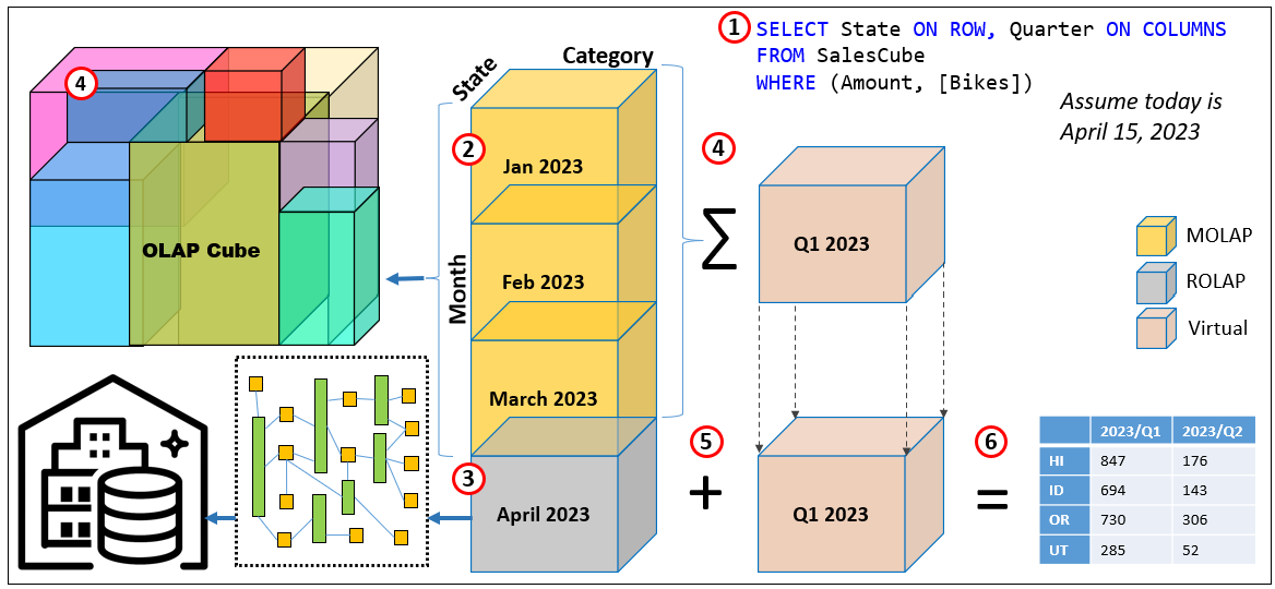
Aggregations are also partitioned into smaller exclusive chunks by some key. They can be managed at the partition level. That means we don’t need to re-process entire partitions. For example, partition by Month, persist what’s stable (MOLAP), and keep the current month as ROLAP for freshness. Quarter totals come from adding months, not from building separate quarter aggregations.

Figure 4 illustrates this query resolution process:

1. Query SELECT State ON ROWS, Quarter ON COLUMNS FROM [SalesCube] WHERE ([Amount],[Bikes]) returns a State × Quarter matrix. Assume today is Apr 15, 2023.
2. MOLAP partitions (persisted). The cube is partitioned by Month at the grain State × Category × Month, with [Amount] as the measure. These monthly partitions are pre-aggregated and stored (MOLAP).
3. Current ROLAP partition. The latest month (here April 2023) is a ROLAP partition. In May, April is processed into MOLAP and a new “current” ROLAP partition is created.
4. Roll-up at query time. For Q1 2023, the engine simply adds the MOLAP monthly partitions (Jan–Mar). For Q2 2023 (so far), it reads April directly from the warehouse via ROLAP.
   No quarter-level aggregation is needed—quarters are computed virtually by summing months.
5. Combine. The ROLAP April result and the sum of Q1 MOLAP months are combined to form the requested quarters.
6. Result. Return a 2D matrix: rows = State, columns = 2023/Q1 and 2023/Q2 (Q2 currently equals April only), with Amount in the cells.

User Need for Lowest-Level Data

Data scientists usually require low-granularity data, often at a high cardinality case level (ex. millions of customers or tens of millions of Web page visits), resulting in very large row counts. The ML algorithms themselves need this detail so they can iterate—experimenting with different sets of features and hyperparameters. In some cases, even more granular, leaf level, transactional data is required, such as individual events or records, to support alternative ways of calculating scores or metrics.

Some traditional BI analysts (less calc-heavy than data scientists) also require the delivery of raw data rather than aggregated results. Sometimes this is simply habit, a carryover from decades before BI became mainstream—perhaps even before Excel became mainstream. Today, it’s more often about the ability to dig deeper. The risk of only receiving highly processed data is that it may have been improperly cleansed—or important signals may have been lost in cleansing. This is where a Data Vault can help preserve raw data lineage. But many of the same user needs could also be addressed with drill-through to the underlying detail, a standard feature of OLAP.

But it’s not a binary choice between raw data and aggregated values. This is the primary issue between OLAP cubes versus Spark (Databricks). For example, a data scientist might request data at the level of page view clicks. It could be that a feature of the page view click is the average time spent of the page—which consists of the aggregation of the time spent on that page divided by the count of hits on that page.

Pre-aggregated OLAP gives us the speed and determinism that BI—and now AI agents—live on. Most enterprise questions are still slice-and-dice over additive measures, and cubes answer those very quickly. The tension shows up when the only data available to modelers is already rolled up (store-week averages, region totals, vendor “health scores”, etc.). At that point you’ve inherited someone else’s assumptions—how prices were averaged, which events were grouped into a “session”, which costs were allocated where. The result is classic lost signal: dispersion disappears, event order collapses into counts, and fat tails get smoothed away. That’s why data scientists push back; not because OLAP is obsolete, but because certain questions require the facts where they’re born before any combining, binning, or allocating.

Concrete examples of metrics that data scientists might want to calculate with alternative methods:

• Retail elasticity & promos: Store-week averages hide coupon mix and price dispersion, leading to wrong own/cross-price elasticities and phantom cannibalization.
• Digital journeys: Daily counts by page look fine, but intent lives in paths (A→B→C) and dwell time, not in marginal totals.
• Manufacturing yield: Line/day defect rates can look stable while a single tool drifts; only unit-level telemetry plus process settings reveal the culprit.
• Claims severity / warranty costs: Region means blur heavy tails and confound driver/product mix; tail modeling needs the individual claim.
• Composite labels: A vendor’s “customer health score” is convenient, but un-auditable; teams need the underlying usage, tickets, SLAs, and surveys to build their factors.

With that context, here’s why leaf-level matters and which measures belong there versus in the cube.

Leaf-level means the grain where facts are born—one transaction/event/claim before anyone collapses it to customer, store-week, or region. Pre-aggregated OLAP shines for additive slice-and-dice, but once you roll up you lock in someone else’s choices (averages, bins, allocations) and lose dispersion, order, and basket context. That’s why data scientists sometimes insist on leaf rows: they need to derive their factors, not inherit non-decomposable composites.

Table 2 lists a few examples of measures that require leaf-level data.

Measure (example)	Needs leaf-level?	Why	OK as OLAP sum?	Caveat / allocation note
Effective price dispersion (per line: price_paid / qty)	Yes	Coupons/price dispersion drive elasticity; averages erase variance and coupon mix.	No	Aggregated “avg price” is not additive and biases elasticity.
Basket co-occurrence (A with B in same transaction)	Yes	Requires knowing which items shared the same basket; counts by day/store lose pairs.	No	Co-occurrence is a set relation at transaction grain.
Units sold (qty)	No	Additive across any slice.	Yes	Safe and natural for cubes.
Discount amount (per line)	No	Additive; rolls up cleanly.	Yes	Still record at line grain; promotion attribution across items may differ.
Shipping/overhead cost (order/store-week totals)	Usually	Sum is easy at order or store, but slicing by product needs allocation.	Looks additive	Without a defensible allocation rule, product-level views mislead.

Use leaf rows for price/basket/sequence features; let the cube answer the additive stuff fast—and tag measures like shipping/overhead as allocation-sensitive so agents know when they’re stepping off solid ground.

Conclusion

I mentioned earlier that OLAP cubes aren’t the answer to everything. Data technologies must meet many conflicting goals. We could create a product that is at best a compromise of all those competing goals—or we can create a team of data engines, each architected for a specific core capability. It would team as a system of specialists, loosely coupled but connected in deliberate ways.

Each engine specializes and is optimized for its respective scenarios. Each specialist will be endowed adjacent capabilities—not as deep as its core—which cover the Pareto majority of use cases. This goes for analytics platforms as well as what will be AGI systems.

This gives resilience—alternative routes, and a modest level of component independence. If one specialist is unavailable, another can step in as a backup, albeit not as good, for most needs or at least keep the system functioning until the specialist is back.

It’s the same reason we value a hospital staffed with many doctors, each a specialist in their own field. A cardiologist doesn’t do brain surgery, and a neurologist doesn’t perform knee replacements—but if a patient first sees the wrong doctor, that specialist can still do some triage until the right one is available. The combination of focused expertise and overlapping coverage is far stronger than one overworked generalist trying to do it all.

In data systems, the same rule applies. A monolith may look neat on paper—a sleek, all-in-one brute—but it becomes brittle and harder to maintain over time. A network of purpose-built engines—cubes, data warehouses, data lakes, ML platforms, event-driven architecture, communication standards, and now even LLMs—gives us both strength in specialization and flexibility in combination.

Part 3 Preview – A Couple of Examples of What’s to Come

In Part 3, I’ll dig into some of the critiques of MOLAP—questions about scalability, brittleness, and whether we really need “all the data.” I’ll also explore how sampling and smarter partitioning open new ways to tackle those challenges. Here are preview examples of topics I’ll address.

Cubes are Brittle

A common critique of OLAP cubes is that they’re brittle—once processed, they can quickly become stale as the world changes. But brittleness can be managed by partitioning data by volatility: history that never changes, near-history that rarely changes, and the current partition where updates occur. Cubes only need reprocessing when rows in those partitions change, giving clear triggers for maintenance.

AI can further reduce overhead by predicting which domains are most likely to change, allowing proactive, targeted reprocessing rather than rebuilding wide swaths of data. In short, history doesn’t change—only our interpretation does—and with the right design, cubes can evolve gracefully with it.

I Hate MDX

So many people hated MDX back when I taught SSAS MD! To me, it’s one of the most elegant languages—right up there with Prolog. The query languages behind Kyvos—MDX and DAX (modeled after Excel functions)—are elegantly versatile, capable of far more than just aggregating additive measures. A clue to their depth is that even the most complicated formulas using include mostly, if not all, sums and counts—just think of all the ∑ symbols scattered across those intimidating equations. Additionally, Kyvos does support a form of SQL as well!

Do We Really Need All the Data?

Modern BI/analytics systems already perform comfortably on data sets under ~200 million rows, which is sufficient for most business domains. While IoT and AI are pushing enterprises toward “billions to trillions” of events, the truth is that for normal business analysis, sampling down to hundreds of millions of rows is usually enough to preserve meaningful patterns.

If we lean on sampling, many of the classic arguments for MOLAP pre-aggregation weaken—since smaller cubes can answer queries fast without elaborate aggregation designs. One way forward is to pair sampled cubes with full cubes: the sampled version for fast exploratory analysis, and the full version for exact reporting. Sampling flags within a single cube are another option, but multiple sampled cubes give more flexibility.

The point is that sampling provides a practical balance: fast queries for exploration, with the ability to requery against the full cube when exact figures are needed. This opens the door to mitigating several issues with pre-aggregated OLAP—topics I’ll explore next in Part 3.

Notes

• This blog is Chapter VIII.5 of my virtual book, The Assemblage of Artificial Intelligence.
• Time Molecules and Enterprise Intelligence are available on Amazon and Technics Publications. If you purchase either book (Time Molecules, Enterprise Intelligence) from the Technic Publication site, use the coupon code TP25 for a 25% discount off most items.