
This article is a supplement to my new book, Semantic Webs of Meaning: Building Contextual Knowledge Graphs for Deduction and Integration published by Technics Publications (on Amazon) . This is an extension to the topic, Machine Learning Models as Data Products, on page 173. In that topic, iris.py is an example of a Python program that creates an ML model (a k-means cluster created from the iris data set) and converts it into an RDF/turtle file. In this article, I wish to offer an example of creating related graphs in a distributed manner.
This article is Part 3 of the series, Inductive Meets Deductive:
- Machine Learning Models in Knowledge Graphs discusses the serialization of ML models (mostly decision trees, clusters, and association) into KG form. Deployed ML models are really a type of business rule, which affects the business. Therefore, its inclusion is critical.
- Jena (Fuseki) Rules for Iris for a tutorial on applying the k-means model into the Jena Fuseki graph DB using Jena Rules.
- Web of Functions (Transformations).
- Re-linking retrained models (~October 2026).
- Implementing decision forests (~October 2026).
- Implementing an ML model trained on the association/arules algorithm (~November 2026).
- Implementing regression, neural networks, and FFT models as rich properties (~December 2026).
If you haven’t read Semantic Webs of Meaning or aren’t familiar with semantic web technology, I advise reading at least the first article, Machine Learning Models in Knowledge Graphs, before continuing with this one.
Notes:
- Some of the figures are very busy. For a full view, click on the Figure, and hit the Browser’s back arrow to return to the this article.
- If purchasing the book from the Technics Publications website, use the code TP25 for a 25% discount.
- The file, iris_rdf.rdf, should really be iris_rdf.ttl. This example has been a part of my “presentation” arsenal for years. Back then, that was the file name, and it got into the book with that name.
- In the context of knowledge graphs, ML models are probabilistic, which does contradict the desire for deterministic answers. For the most part, ML models output answers with probabilities, but they will still be the same answer and probability for the same input … until the model is retrained, which we’ll talk about in Part 4.
Web of Functions
Up until this blog, I’ve presented my old work in Map Rock (ca. 2011) as the predecessor to the Tuple Correlation Web (TCW). However, the TCW is just one side of the coin. The TCW is intended to integrate islands of data through the ubiquitous dimension of time. This was extremely tedious without LLM assistance.
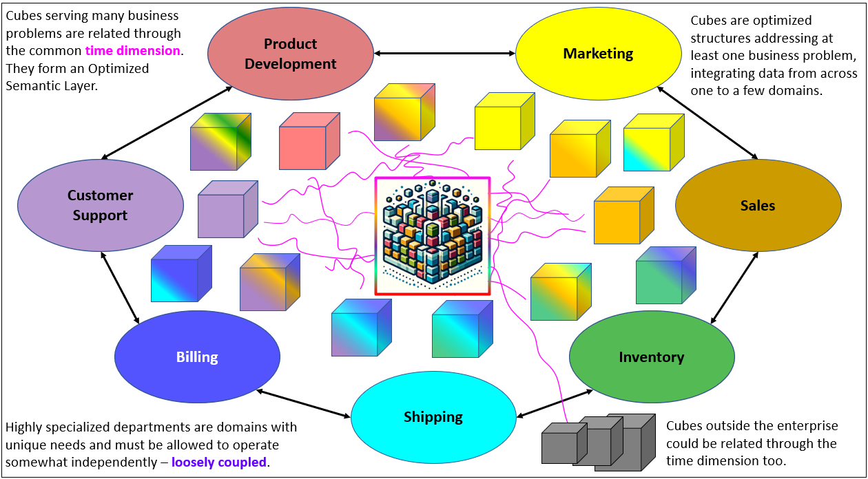
Figure 1 illustrates the idea of integrating many domain-oriented BI data sources (the cubes) through the ubiquitous, common dimension of time—even without other common dimensions (ex. customer, product, location). There is much we could glean from time-oriented measures such as Pearson/Spearman correlations and date-based conditional probabilities.
The other side of the coin, the subject of this blog, is a map of functions linked through their outputs and inputs. It’s really what put the “map” in Map Rock—the map of transformations, the knowledge graph of the instigation (inputs) and result (outputs) of interactions. The functions were mostly machine learning models, growing in number with the rise of data science around that 2011 timeframe.
A Web of Functions is formed when the inputs and outputs of computational functions are linked via semantically identified data elements. The graph can then reveal not only pipelines that have already been built, but functions that could be composed because one produces what another requires.
A function maps inputs to an output. The function can be as simple as a mapping table, an equation, or a procedure ranging in complication from a few steps (like a decision tree) to even millions of steps (like the aggregation of millions of rows).
There is a strict definition of a function. One of its most important properties is that a given input always returns the same output. This is more precisely called determinism, while a function that also has no side effects is called a pure function. In real life, that may not appear to be intuitively true. If I ask my friend what his favorite drink is, I might expect the same answer every time, yet the answer can change. That does not necessarily break the definition of a function; it may mean that I have failed to identify all the inputs. His answer might also depend on the time, place, mood, available choices, or even how I phrase the question. What looks like inconsistency may actually reveal hidden inputs. In a Web of Functions, those inputs—and any effects the function has on the world—should be made explicit whenever they matter.
Note: When a function changes, the same inputs may map to different outputs. That does not break the definition of a function because different rules constitute a different function, even when it retains the same name. The function should therefore be versioned so that we can “time travel”—identify which rules were in effect at a particular time and reproduce the result they would have produced.
Give function inputs and outputs semantic identities in a KG so existing dependencies, possible compositions, missing transformations, provenance paths, and uncertain mappings can be discovered and reasoned about.
Figure 2 illustrates an example of a web of functions.
- Iris is the entity presented to the first function. In this example, the input could be a photograph of an iris rather than measurements that have already been recorded.
- Sepal, Petal Measurement is a black-box function. Its internal image-processing or AI logic is not modeled here; only its input and outputs are described.
- Petal Length and Sepal Length are separate data-element individuals with their own IRIs. They are outputs of the measurement function and inputs to the Iris KMeans model.
- Iris KMeans Model accepts the required measurements and applies the previously trained clustering model.
- Iris Classification identifies the kind of result produced by the model. Its possible values are the three learned iris clusters, and the same node can serve as an input to another function.
- Iris Pricing combines the iris classification with customer and delivery information to calculate a price.
- Customer Type and Delivery Method are input data elements shared by the Iris Pricing and Ginger Pricing functions.
- Quoted Price is the common output data element of the pricing functions. It identifies the kind of result produced, not a particular dollar amount.
- Ginger Pricing combines a ginger classification with the shared customer and delivery inputs to produce a quoted price.
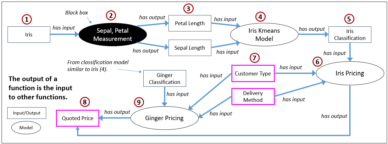
Figure 3 shows a less cluttered version of Figure 2—four functions with just their inputs and output(s). The intent is to highlight that ML models, like other semantic web resources, can be built independently and linked via IRI:
- The Sepal, Petal Measurement function accepts an iris and produces the measurements needed by the classification model.
- The Iris KMeans model accepts the measurement features and produces an iris classification.
- The Iris Pricing function accepts the iris classification, customer type, and delivery method and produces a quoted price.
- The Ginger Pricing function follows the same pattern, accepting a ginger classification and the shared pricing inputs and producing a quoted price.
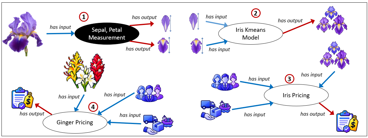
It’s important to remember that the properties of the ML models are not displayed in Figures 2 and 3 as described in Machine Learning Models in Knowledge Graphs. That would result in a very busy incomprehensible illustration.
The Black Box Function
Decision Forests, association rules, sequences, k-means clusters, and even the various encoded forms of IF-THEN type of rules (ex. SWRL, Prolog) are all relatively simple to diagram in graph form, again, as I describe in Machine Learning Models in Knowledge Graphs.
In Figures 2 and 3, there is a “black box function” (Sepal, Petal Measurement), by which I mean that we don’t intend to map its internal working in the knowledge graph. This is more like “rich properties” I describe in Appendix F – Rich Properties, properties that we know contain much knowledge but we choose not to map it out. This could be for many reasons:
- It’s not at all feasible. For example, a “function” could be a human manager who approves a discount, or an LLM with billions to trillions of “parts”. The human brain is the black box of all black boxes.
- It’s feasible, but too cumbersome in relation to the value it provides. For example, a function written in Python or Java. Yes, we could break it down into a graph form (i.e. Abstract Syntax Tree), but it’s not necessary since it’s understandable by programmers and LLMs today.
- Taking #2 further, it could be an entire system. For example, a BI system that gets the answer to: “What is my total sales of bikes in Arizona?”
- The mechanisms are unavailable to us—private, guarded, obfuscated, and very often purposefully deceiving to throw us off course with misinformation (ex. camouflage used by all predator and prey).
The notion of simply “it’s not important” isn’t a valid reason in itself to represent a model as simply a black box. Everything is connected and the entire idea of intelligence is to see and analyze beyond the box of what we know. The articulation of the mechanics of what is currently a black box, that could feasibly be described, should be considered a “backlog item”.
Prior and Similar Work in the Conceptual Neighborhood
My path to the Web of Functions began with the Maps feature I built into Map Rock in the early 2010s. It assembled rules, goals, BI objects, predictions, and other elements into navigable maps of relationships. It was not expressed as an RDF ontology of functions, but the underlying idea of mapping functions and the relationships among them was already there. This article returns to that Map Rock work and recasts it using IRIs and knowledge graph relationships.
Figure 4 is a rare snapshot of the “Maps” view of Map Rock I took a couple of years ago (after over a decade in mothballs).
- The Maps tab of Map Rock. A map is a web of functions (mostly ML models) and correlations.
- The Discover tab of Map Rock, described in Map Rock – 10th Anniversary and Some Data Mesh Talk.
- Selection of authored Maps.
- Correlations discovered in the Discover tab (2).
- An early attempt at a user-editable graph interface in 2011.
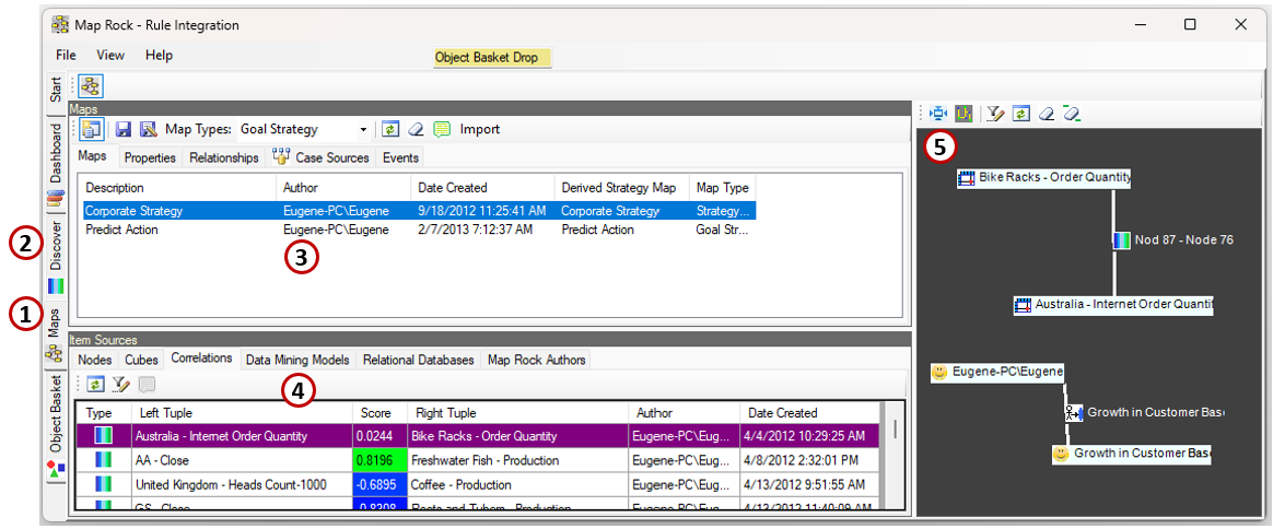
The graph displayed in item 5 of Figure 4 admittedly does not look much like the graph interfaces we expect today. In 2011, drawing nodes and edges was not the hardest part. The difficulty was finding a graph control that behaved like a complete application control. I needed users to add, move, connect, delete, select, and edit graph objects; invoke functions from them; manipulate the view; and save the resulting map. Grid controls of that era already provided a rich set of editing, navigation, and data-binding capabilities, but finding an equivalent graph control—and one I could realistically afford and integrate—was much harder. In fact, that is why item 4 shows a grid view.
Building all of those capabilities myself would have amounted to developing another major product inside Map Rock. Combined with the SCL language, machine learning integration, BI objects, correlation discovery, and everything else Map Rock attempted to do, it became too much for one person who needed to make a consistent living. The graph visualization therefore remained rudimentary, but the underlying idea of mapping connected functions was already there.
My Own Lineage: APBIA and Reps
Map Rock’s “Maps” tab shown in Figure 4 was the original implementation of what I am referring to as “Web of Functions” in this blog. By 2011, it was already bringing rules, goals, BI objects, machine learning models, predictions, and correlations into a navigable graph.
When Micron announced its Automata Processor in late 2013, I recognized it as what I needed to carry out the querying of the “Maps” tab at scale—to carry that idea beyond mapping and into massively parallel execution. I called the proposal APBIA (to Micron)—the Automata Processor Business Intelligence Appliance (ca. 2014). The idea was to collect models from across an enterprise, convert those suited to the task—such as decision trees, association rules, and sequence models—into nondeterministic finite automata (NFA), and load thousands of them onto a bank of Automata Processors. The same stream of symbols could then be presented to all the models in parallel.
I first wrote about the processor in Micron’s Automata—A Rare Big Thing Out of Boise and described APBIA. I did finally describe the NFA design more fully in I’m Speaking at DMZ 2025—Sample from My Talk—NFA. When the Micron path “stalled”, I pursued a software implementation (C#) called Reps, which I revisit in Reptile When the Micron path did not develop further, IIntelligence: An AI Summer for CEP.
It might be interesting to read a similar take at the approach: Towards Machine Learning on the Automata Processor | Eric Jonas
In this lineage, Map Rock supplied the original map, while APBIA and Reps explored how many mapped functions could be translated into a common form and executed together. The present Web of Functions returns to the map and adds semantically identified inputs and outputs so that those possible compositions can be discovered in a knowledge graph.
The world is a big place. So, of course over the years, many people work on the same thing unknown to others. Following are a few selected examples of work in this conceptual neighborhood. My apologies for any that I undoubtedly must have missed.
Function Ontology (FnO)
In 2016, Ben De Meester and his colleagues introduced the Function Ontology (FnO). FnO describes functions independently of the programming language or technology implementing them and distinguishes among functions, input parameters, outputs, algorithms, executions, implementations, and the problems functions solve. The May 12, 2023 FnO specification also includes vocabularies for mapping implementations and composing functions by connecting outputs to parameters. The specification remains an unofficial draft rather than an endorsed standard.
See: An Ontology to Semantically Declare and Describe Functions, ESWC 2016, Ben De Meester et al.
The emphasis of this article is the Map Rock idea carried into Semantic Webs of Meaning: semantically identified data elements make the output of one function visibly available as the input to another, while any required mapping or transformation becomes another function in the graph.
Another “Web of Functions”
While researching other work, I discovered that Maurizio Atzori used “Web of Functions” in 2014–2015 for interoperable higher-order functions in pure SPARQL: a function advertised by URI, executed on the endpoint that implements it, callable without vendor-specific extension functions. That is a federation problem for SPARQL. This article is a capability-mapping problem for enterprise models, rules, and adapters. Same words, different graph.
Semantic Web services and Workflow Provenance
Before FnO, OWL-S, WSMO, and SAWSDL already advertised software capabilities by typed inputs and outputs and asked a planner to compose them. The objects were Web services. The pattern was the same: ports, not source code, are what make composition searchable.
PROV-O, P-PLAN, and OPMW already describe plans and runs. If a Web of Functions is going to support time travel—replay what a quoted price was under yesterday’s function version—it should record executions in those vocabularies rather than invent another provenance dialect. The function graph says what can be done. Provenance says what was done.
Wikifunctions and Operational Catalogs
Wikifunctions is a collaboratively edited library of functions intended to render Abstract Wikipedia into natural languages. It is a global commons of callable operations. A Web of Functions in the sense of this article is local and messy: the pricing function that only Sales trusts, the measurement function that lives in a contractor’s notebook, the human approval that never acquired an IRI.
Operational platforms already catalog models and interfaces: MLflow and similar model registries, feature stores, pipeline DAGs, data-product registries in a data mesh. They are good at “here is a model and here is its schema.” They are weaker at treating the adapter as a first-class, versioned function, and they do not sit beside a correlation web that says which tuples actually move together in the business. The Web of Functions is not a replacement for those registries. It is the semantic layer that makes their interfaces composable with everything else the enterprise can already do.
Walkthrough
Let’s look at how some of this will look in Protégé—up to the point of an ML model with the input and outputs resources that could be recognized by other types of functions (broader than just ML models, ex. functions deployed as AWS lambda functions or parameterized SQL Server stored procedures).
Figure 5 illustrates the ontologies that comprise the demo.
- Open protege with iris_rdf.rdf. This is the base ontology containing the iris model, its learned clusters, and the original iris concepts.
- Import iris_rdf_world_links.ttl. This file connects local iris resources to related external identifiers.
- Import iris_web_of_functions.ttl. This file adds the computational functions and the semantically identified input and output data elements.
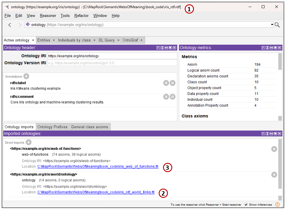
Figure 6 shows how to view the input and outputs of the Iris KMeans model.
- The Individuals view displays the specific nodes contained in the combined ontologies.
- Iris KMeans model is selected as an individual. It is the hub that connects the model to its inputs and output.
- The has output assertion links the model to the Iris classification data-element individual.
- The has input assertions link the model to four separate feature individuals: iris petal length, iris petal width, iris sepal width, and iris sepal length.
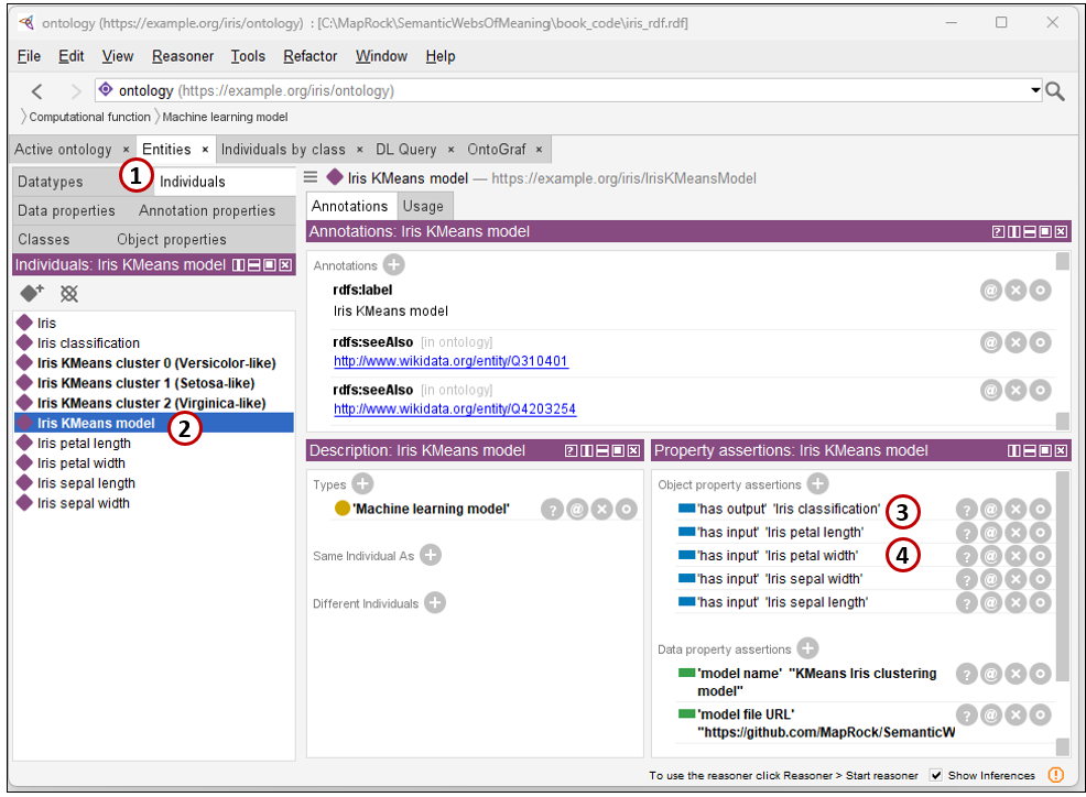
Figure 7 takes a closer look at the output class of the Iris KMeans model.
- Iris classification is selected as an individual representing the model’s output data element.
- The Usage tab displays statements in which the selected individual participates.
- The has possible value assertions link the output to the three learned cluster nodes: Virginica-like, Setosa-like, and Versicolor-like. The output also specifies that it describes an Iris.
- The reverse usage statement shows that Iris KMeans model has Iris classification as its output.
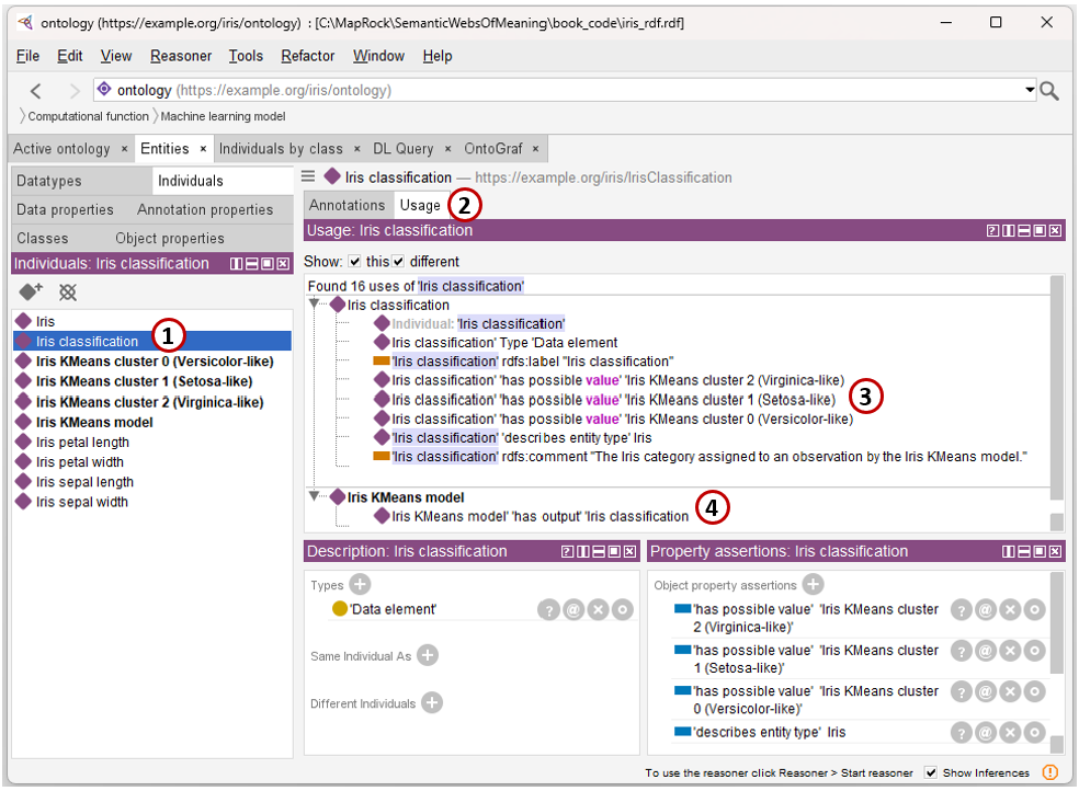
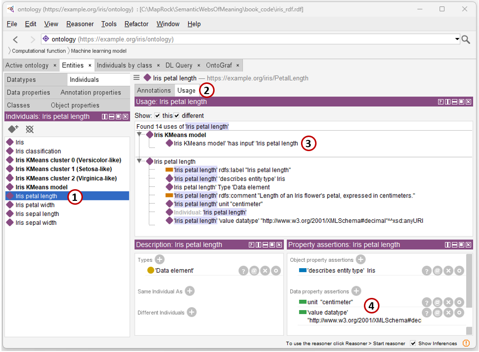
Figure 8 looks closely at one of the iris classifications, one of the possible outputs.
- Iris petal length is selected as one of the model’s input data-element individuals.
- The Usage tab gathers the statements involving this feature node.
- The reverse usage statement shows that Iris KMeans model has Iris petal length as an input.
- The feature’s properties specify its meaning and expected value: it describes an Iris measurement, uses centimeters as its unit, and expects an xsd:decimal value.
Translations
Giving every input and output an IRI establishes its identity inside the graph. It does not mean that another organization, model, or knowledge graph will use the same IRI—or even describe the same thing in the same way. Even a conversation between Noam Chomsky and William F. Buckley Jr.—known for precise, articulate speech and careful command of language—would require period clarification of terms.
Another source may use a different label, a different IRI, a broader concept, a different unit of measurement, or a value that must be interpreted before it can be used. These are not all the same kind of relationship.
A good first question is:
Are these two resources the same thing, similar things, or values that can be transformed into one another?
| Situation | RDF/OWL/SKOS expression |
|---|---|
| Another name for the same resource | skos:altLabel |
| Related information, without claiming equivalence | rdfs:seeAlso |
| Exactly the same individual | owl:sameAs |
| Classes with the same extension | owl:equivalentClass |
| Concepts that closely align | skos:exactMatch or skos:closeMatch |
| One concept is broader or narrower | skos:broadMatch or skos:narrowMatch |
| Mapping depends on context or probability | A mapping assertion individual |
| The value must be converted or interpreted | Another computational function |
Another Label is not Another Identity
The simplest case is a second name for the same data element. The data element keeps one IRI, but it can have several human-readable labels.
ex: <https://example.org/iris/> . skos: <http://www.w3.org/2004/02/skos/core#> .ex:PetalLength skos:prefLabel "Iris petal length"@en ; skos:altLabel "petal length"@en ; skos:altLabel "length of iris petal"@en .
skos:prefLabel identifies the preferred label for a language, while skos:altLabel supplies recognized alternatives. SKOS also provides skos:hiddenLabel for misspellings, obsolete spellings, and other forms that may help search but should not normally be displayed. The SKOS specification permits these labels to be applied to any RDF resource, including the data-element individuals in this example.
These labels do not create new input or output nodes. They are different names for ex:PetalLength.
Another IRI Makes a Stronger Claim
The next case involves two IRIs. The current iris_rdf_world_links.ttl uses a conservative relationship:
wd: <http://www.wikidata.org/entity/> . rdfs: <http://www.w3.org/2000/01/rdf-schema#> .ex:IrisKMeansCluster_0 rdfs:seeAlso wd:Q164844 .
This says that the Wikidata resource may provide useful information related to the cluster. It does not say that the two resources are identical.
That distinction matters. ex:IrisKMeansCluster_0 is a result produced by a particular trained model. Its dominant species in the training data is Iris versicolor, but the cluster itself is not the botanical species. Therefore, this would be too strong:
# Do not make this assertion.ex:IrisKMeansCluster_0 owl:sameAs wd:Q164844 .
owl:sameAs means that two individual IRIs identify the same individual and can be substituted for one another without changing the ontology’s meaning. It is not a general-purpose “these seem alike” relationship. That is the formal meaning assigned by OWL 2.
A good test is to ask whether the two nodes could be merged, along with all their properties, without losing a distinction. If not, they are not owl:sameAs.
For vocabulary alignment, SKOS offers weaker choices:
partner: <https://example.com/partner-vocabulary/> .ex:PetalLength skos:Concept ; skos:exactMatch partner:IrisPetalLengthCentimeters .ex:IrisClassification skos:Concept ; skos:closeMatch partner:IrisSpeciesCategory .
skos:exactMatch expresses a high-confidence conceptual match. skos:closeMatch says that the concepts are similar enough for some uses but should not be treated as universally interchangeable. Importantly, skos:exactMatch is transitive, while skos:closeMatch is not. The distinction is described in the SKOS mapping specification.
Neither property automatically proves that two function interfaces are operationally compatible. Their datatypes, units, possible values, cardinality, and entity types must still be examined.
Colloquial Names May Require Context
The ginger example shows why a literal name may be insufficient.
GBIF lists Hedychium gardnerianum with vernacular names including “Kahili ginger” and “Kahili ginger lily”. However, kāhili also refers to a Hawaiian feather standard associated with royalty. The string by itself therefore does not identify a single concept. GBIF and the Kapiʻolani Community College glossary illustrate the two meanings.
The unambiguous plant name can be recorded normally:
ex:KahiliGinger skos:Concept ; skos:prefLabel "Hedychium gardnerianum" ; skos:altLabel "Kahili ginger"@en ; skos:altLabel "Kahili ginger lily"@en ; rdfs:seeAlso <https://www.gbif.org/taxon/3JZPN> .ex:KahiliFeatherStandard skos:Concept ; skos:prefLabel "kāhili"@haw ; skos:prefLabel "feather standard"@en .
The bare word “kahili” should not automatically be made an alternate label for the plant in a vocabulary that also discusses Hawaiian culture. Its meaning depends upon context.
When the label itself requires a source, region, time period, or usage note, SKOS-XL can turn the label into an identifiable resource:
skosxl: <http://www.w3.org/2008/05/skos-xl#> . dcterms: <http://purl.org/dc/terms/> .ex:KahiliPlantLabel skosxl:Label ; skosxl:literalForm "kahili"@en ; ex:usedInContext ex:HawaiiPlantCatalog ; dcterms:source ex:LocalNurseryVocabulary .ex:KahiliGinger skosxl:altLabel ex:KahiliPlantLabel .
This is appropriate when “kahili” is an accepted plant label within a clearly defined vocabulary. It still should not be treated as an unconditional global identity.
Probabilistic Mappings Should be Individuals
A mapping produced by an LLM or another probabilistic process should not immediately become an owl:sameAs assertion. It should first become a mapping proposal with its own IRI.
prov: <http://www.w3.org/ns/prov#> . xsd: <http://www.w3.org/2001/XMLSchema#> .ex:Mapping_2384 ex:MappingAssertion, prov:Entity ; ex:sourceLexicalForm "kahili"@en ; ex:mapsTo ex:KahiliGinger ; ex:proposedRelation skos:closeMatch ; ex:requiredContext ex:HawaiiPlantCatalog ; ex:confidence "0.78"^^xsd:decimal ; ex:mappingStatus ex:Proposed ; prov:wasGeneratedBy ex:NameResolutionRun_2384 .
The mapping can now be reviewed, rejected, approved, replaced, or limited to a particular context. Its provenance and confidence are not hidden inside a comment.
A sufficiently trusted mapping process could later materialize a SKOS relationship. It should not materialize owl:sameAs merely because it exceeded a probability threshold. Probability is evidence for a claim, not the same thing as logical identity.
A Transformation is Another Function
Some inputs and outputs do not merely have different names. Their values must be changed.
Suppose another function produces iris petal length in inches, while the Iris KMeans model expects centimeters. Those data elements are related, but they are not identical.
Using an IRI for the expected unit makes that difference machine-readable. The existing string value can remain for display, but a unit IRI can be added:
qudt: <http://qudt.org/schema/qudt/> . unit: <http://qudt.org/vocab/unit/> .ex:expectedUnit owl:ObjectProperty ; rdfs:range qudt:Unit .ex:PetalLength ex:expectedUnit unit:CentiM .ex:PetalLengthInches owl:NamedIndividual, ex:DataElement ; rdfs:label "Iris petal length in inches" ; ex:valueDatatype "http://www.w3.org/2001/XMLSchema#decimal"^^xsd:anyURI ; ex:expectedUnit unit:IN ; ex:describesEntityType ex:Iris .
unit:CentiM and unit:IN identify the centimeter and inch rather than relying upon locally chosen strings.
The bridge between them is a function:
ex:TransformationFunction owl:Class ; rdfs:subClassOf ex:ComputationalFunction .ex:PetalLengthInchesToCentimeters owl:NamedIndividual, ex:TransformationFunction ; rdfs:label "Convert iris petal length from inches to centimeters" ; ex:hasInput ex:PetalLengthInches ; ex:hasOutput ex:PetalLength ; ex:expression "centimeters = inches * 2.54" .
The graph can now discover a valid path:
Measurement function → Petal length in inches → Inches-to-centimeters transformation → Petal length in centimeters → Iris KMeans model
The conversion is not hidden in integration code. It has an IRI, defined inputs and outputs, and a place in the Web of Functions.
The same pattern can be used for categorical mappings. A local ginger-name resolver could consume a name, photograph, and locale, then produce a ginger classification and a confidence value:
ex:LocalGingerNameResolver owl:NamedIndividual, ex:TransformationFunction ; rdfs:label "Resolve a local ginger name" ; ex:hasInput ex:LocalPlantName, ex:PlantPhotograph, ex:GeographicContext ; ex:hasOutput ex:GingerClassification, ex:MappingConfidence .
This is particularly important for ambiguous names. The word “kahili” alone may be insufficient, but “kahili,” a photograph of the flower, and a plant-sales context may provide enough evidence for classification.
An execution of the resolver can also be recorded with PROV-O:
ex:NameResolutionRun_2384 prov:Activity ; ex:executesFunction ex:LocalGingerNameResolver ; prov:used ex:RawPlantDescription_2384 ; prov:generated ex:ResolvedGingerClassification_2384 .ex:ResolvedGingerClassification_2384 prov:wasDerivedFrom ex:RawPlantDescription_2384 .
PROV-O describes an activity as something that can consume, process, or transform entities and generate new entities. This makes it suitable for recording the execution and provenance of a transformation, while ex:ComputationalFunction describes the reusable function itself. See the PROV-O specification.
SHACL can Check Whether a Direct Connection is Safe
OWL and SKOS describe semantic relationships. SHACL can describe the interface requirements that must be satisfied before one function’s output is directly connected to another function’s input.
sh: <http://www.w3.org/ns/shacl#> .ex:PetalLengthInterfaceShape sh:NodeShape ; sh:targetNode ex:PetalLength ; sh:property [ sh:path ex:valueDatatype ; sh:hasValue "http://www.w3.org/2001/XMLSchema#decimal"^^xsd:anyURI ] ; sh:property [ sh:path ex:expectedUnit ; sh:hasValue unit:CentiM ] .
SHACL does not perform the conversion. It determines whether the input/output contract is satisfied. If it is not, the graph can search for a transformation function that bridges the difference.
For example:
PREFIX ex: <https://example.org/iris/>SELECT ?producer ?transform ?consumerWHERE { ?producer ex:hasOutput ?sourceElement . ?transform a ex:TransformationFunction ; ex:hasInput ?sourceElement ; ex:hasOutput ?targetElement . ?consumer ex:hasInput ?targetElement .}
This extends the Web of Functions beyond locating exact shared nodes. It can also locate paths through the transformations that make functions compatible.
The general rule is:
A second label is a name. A mapping is a claim. A transformation is a function.
The graph should not pretend that two inputs or outputs are identical when work is required to move from one to the other. That work is itself part of the Web of Functions.
Testing the Web of Functions
To try out this work, we’ll use Jena Fuseki:
- If necessary, perform Steps 1–4 in Installing and Running Apache Jena Fuseki. These steps start Fuseki with an in-memory dataset named
/kg. - Keep the PowerShell window running, open
http://localhost:3030, and select the/kgdatabase. Open the add data tab for/kg. - Leave Dataset graph name blank, select iris_web_of_functions_complete.ttl, and click upload all. This is a standalone Turtle file, so no other RDF file is required for the queries in this example.
- Click on the query tab in order to enter test SPARQL queries.
Here are a couple demonstrations beyond the transformation query.
Discover functions that can be directly connected
This finds cases where one function’s output is another function’s input.
PREFIX ex: <https://example.org/iris/>PREFIX rdfs: <http://www.w3.org/2000/01/rdf-schema#>SELECT DISTINCT ?producerLabel ?dataElementLabel ?consumerLabelWHERE { ?producer ex:hasOutput ?dataElement . ?consumer ex:hasInput ?dataElement . FILTER (?producer != ?consumer) ?producer rdfs:label ?producerLabel . ?dataElement rdfs:label ?dataElementLabel . ?consumer rdfs:label ?consumerLabel . FILTER (LANG(?producerLabel) = "en") FILTER (LANG(?dataElementLabel) = "en") FILTER (LANG(?consumerLabel) = "en")}ORDER BY ?producerLabel ?dataElementLabel ?consumerLabel
This should reveal connections such as:
- Sepal and petal measurement → Iris petal length → Iris KMeans model
- Iris KMeans model → Iris classification → Iris pricing
- Local ginger name resolver → Ginger classification → Ginger pricing
- Inch-based measurement → Petal length in inches → conversion function
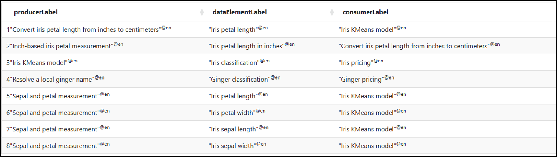
The output contains eight direct handoffs between functions. Each row identifies a producing function, the data-element node it produces, and a function that accepts that same node as an input. The four iris measurements (5-8) connect the Sepal and Petal Measurement function to the Iris KMeans model, while Iris Classification (3) connects the KMeans model to Iris Pricing.
Ginger Classification (4) similarly connects the local-name resolver to Ginger Pricing.
The two petal-length conversion rows (1 and 2) are particularly important: together, they show the inch-based measurement feeding the inches-to-centimeters transformation, which then produces the centimeter-based Petal Length required by the Iris KMeans model. The query returns direct connections rather than entire pipelines, but those connections can be assembled into longer paths.
Find everything that can influence the quoted price
This uses a SPARQL property path to work backward through any number of functions.
PREFIX ex: <https://example.org/iris/>PREFIX rdfs: <http://www.w3.org/2000/01/rdf-schema#>SELECT DISTINCT ?upstreamElement ?elementLabelWHERE { ?upstreamElement (^ex:hasInput/ex:hasOutput)+ ex:QuotedPrice . OPTIONAL { ?upstreamElement rdfs:label ?elementLabel . FILTER (LANG(?elementLabel) = "en") }}ORDER BY ?elementLabel
Figure 10 lists the results.
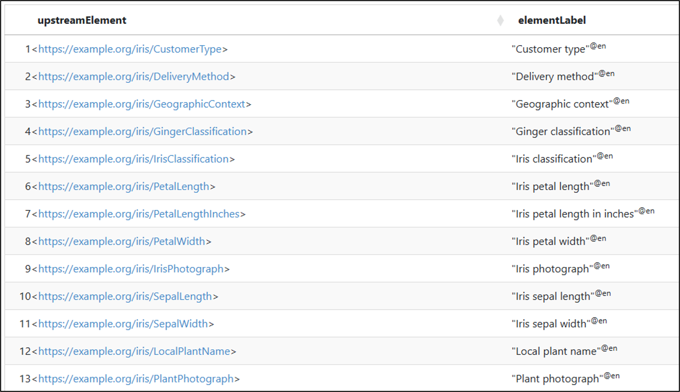
The output lists thirteen data elements that can directly or indirectly influence Quoted Price. Customer Type (1), Delivery Method (2), Iris Classification (5), and Ginger Classification (4) are direct inputs to a pricing function. The remaining rows are farther upstream: iris photographs (9) and measurements (6, 8, 10, 11) lead to Iris Classification (5), while a local plant name (12), plant photograph (13), and geographic context (3) lead to Ginger Classification (4).
Petal Length in inches (7) also appears because it can be transformed into the centimeter-based Petal Length used by the Iris KMeans model. The query returns data elements rather than functions, and DISTINCT prevents shared inputs such as Customer Type (1) from appearing twice.
Mapping Confidence does not appear because, although the ginger resolver produces it, no function uses it on a path leading to Quoted Price. This is impact analysis over the Web of Functions: it identifies what could ultimately affect a selected output rather than merely what connects to it directly.
The first query discovers composable links. The second performs impact analysis: “What could ultimately affect this output?”
Conclusion
The SPARQL queries at the end aren’t complicated, but the questions they answer are important. What functions can be connected? What transformations can bridge incompatible inputs and outputs? What things, even several steps upstream, can influence a quoted price? Those answers are possible because Petal Length, Iris Classification, Quoted Price, and the other data elements are not just labels in a diagram. They are identified resources with IRIs and described meaning.
A Web of Functions does not require us to pry open every black box or force every function into RDF. It requires us to say enough about what a function needs and what it produces for it to participate in the larger graph. If a unit conversion, name resolution, probabilistic mapping, or other transformation is required, that work should not disappear inside integration code. It is another function, with its own identity and place in the web.
This creates more than a catalog of existing pipelines. It creates a map of enterprise capability. Functions can continue to be developed independently—in Python, ML platforms, BI systems, rule engines, or even performed by people—while their semantically identified interfaces reveal how the pieces already connect and where new compositions are possible.
This also suggests a natural role for what I think of as AI in the loop. An LLM does not need to be the function doing the work; it can sit between functions, interpreting what one function produced, translating it when necessary, evaluating the context surrounding the result, and helping determine which function should receive it next. In that role, AI becomes less another application in the web than connective intelligence among otherwise independently developed capabilities.
This is knowledge even when we choose not to represent the internal workings of every function: knowledge of requirements, results, dependencies, transformations, and possibilities.
The TCW connects observations across time. The Web of Functions connects capabilities through inputs and outputs. One helps us see relationships in what happened, while the other helps us discover what can be done next. Together they complete the two sides of the original Map Rock idea: a map of what the enterprise knows and a map of what it can do with that knowledge.


One thought on “Web of Functions (Transformations)”