
Note: From the “deleted scenes” of my book, Enterprise Intelligence, Technics Publications, 2024.
This addresses a layered approach to building a Tuple Correlation Web (TCW), which can be massive in its full, enterprise-scoped manifestation.
The TCW is primarily an Enterprise Intelligence structure, but it also belongs within the larger idea of my new book, Semantic Webs of Meaning (on Amazon). Its correlations are not “formal ontology” and should not be mistaken for permanent semantic truths [8]. They are empirical knowledge: two qualified measures moved together under a particular method, date range, grain, lag, and set of model versions. When those relationships are represented as knowledge graph entities, their context can be preserved and they can be connected to the KPIs, measures, formulas, business concepts, data sources, insights, and events that give them meaning. The TCW is therefore one of the semantic webs of meaning—one built from observed relationships rather than asserted definitions.
From a KPI in Pain to an Expanding Investigation
This blog describes the procedure for employing the TCW for correlation exploration used to resolve business problems in a “strategic troubleshooting” mode (geared towards novel problems that escapes troubleshooting with known tactics). It begins with Key Performance Indicators (KPI) and progresses through a few stages.
Performance investigations begin when something important is not behaving as intended. Sales falls below target. Inventory turns red. Customer attrition rises. Page-response time approaches an unacceptable level. A KPI has entered pain, and someone wants to know why. The ability to notice and identify “pain” is arguably the purpose of Performance Management and Dashboards.
Dashboards and KPIs are where performance management and BI connect.
That misbehaving KPI gives us a small, meaningful place to begin. From there, the search can widen in rounds, as shown in Figure 1.
- Correlate the distressed KPI tuple with other KPI tuples.
- Expand to ordinary tuples that share informative elements with the strongest KPI relationships.
- Use the Insight Space Graph (ISG) to find inflections, spikes, clusters, stable measures, and other observations involving those tuples.
- Use the timing and context of those insights to introduce new tuples, including tuples from domains that did not share obvious elements with the original KPI.

This turns the ISG and TCW into a feedback loop. The ISG can supply tuples to the TCW, but TCW discoveries can also tell us where to search the ISG.
A KPI Status Is a Tuple
A KPI is not just a freestanding number. A KPI value or status is calculated within a dimensional context. For example:
( Measure = Gross Margin KPI Status, Product Category = Bikes, Region = Northwest, StartDate = 2024-01-01, EndDate = 2024-05-31 )
A tuple is a metric qualified by a set of dimensional members. Change one member and it becomes another tuple. Gross Margin Status for Bikes in the Northwest is not the same tuple as Gross Margin Status for Clothing in the Northwest or Bikes in the Southwest.
This qualification is important because the overall corporate Gross Margin KPI might be healthy while the same KPI for one product category and region is deteriorating. The problem often lives below the grand total.
Time does not necessarily need to appear in the displayed tuple. In multidimensional terms, a tuple that omits a hierarchy is a partial tuple. The missing hierarchy is completed by the applicable default or query context. For a time-series calculation, however, the correlation request deliberately evaluates the subject tuple across a sequence of Date members perhaps the last 52 weeks or 24 months.
Each observation therefore has a date even when Date is omitted from the shorthand used to name the subject tuple. The subject tuple identifies what is being measured; the Date axis supplies the repeated observations:
Gross Margin Status for Bikes, Northwest, 2024-01-01, 2024-05-31 Week 1 -> 0.91 Week 2 -> 0.88 Week 3 -> 0.79 ...Inventory Status for Bikes, Northwest, 2024-01-01, 2024-05-31 Week 1 -> 0.86 Week 2 -> 0.81 Week 3 -> 0.70 ...
These sample values use the convention that a higher status is healthier. The two time-aligned series can now be compared. The correlation calculation must specify the date range, grain, and any lag even when Date is not treated as part of the stable identity of either subject tuple.
KPI status is particularly attractive for the first round because it translates measures with different units into a roughly common language of performance. Revenue, inventory availability, response time, and customer retention have incompatible raw units, but their statuses express how each is performing relative to its intended state.
That assumes the status conventions are consistent. If a higher status means healthy for one KPI and pain for another, the values should be normalized before interpreting the sign of a correlation. Historical KPI formulas and targets must also be preserved. We cannot reconstruct last year’s KPI status accurately using only today’s target or today’s version of its formula.
Pain is the Instigator
KPI dashboards are attention systems. Their purpose is to compress a large enterprise into a small set of measures that warn people when something important needs attention. A “red” KPI (usual visual for a rapidly deteriorating KPI) therefore supplies a natural seed tuple for TCW probing. KPI statuses are pain. For example, the KPI for active customers of bikes in the Northwest for the current quarter might be indicating trouble:
( Active Customer Status, Product Category = Bikes, Region = Northwest, StartDate = '2024-01-01', Enddate = '2024-03-10')
The tuple becomes “lit up”, receiving a high probing priority because it represents current pain rather than background curiosity. The system does not yet know why the KPI is in pain. It only knows where to begin looking. This is a substantial reduction in search space. Instead of asking which relationships among millions of tuples might be interesting, we ask which relationships may help explain one specific condition that currently matters.
Round 1: Correlate KPI Tuples
The first candidate population consists only of KPI tuples. An enterprise might have hundreds or thousands of KPIs when dimensional slices are included, but that is still a manageable subset of the full tuple space. It might consist of a few million relationships, but not billions or trillions.
For the selected time window and grain, the system retrieves the time series for the distressed KPI tuple and compares it with other KPI-status tuples. Existing TCW edges can be reused when their calculation context is still compatible and fresh. Missing or expired relationships are recalculated on demand.
The first pass might find relationships such as (assume implied date range of 2024-01-01, 2024-03-10, the current quarter) as shown in Figure 1.
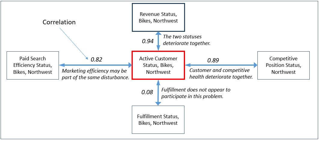
A strong correlation does not mean one KPI affects another. Pearson correlation is symmetric. It tells us that two status series move together or in opposition, not which one is the cause. Directional evidence may later come from time lags, known strategy-map relationships, formula lineage, events, Markov models, domain knowledge, or explicit rules.
Even so, the first round is valuable. It produces a small neighborhood of KPI states, a few plausible hints, that appear to participate in the same business disturbance. It also provides negative evidence. A fulfillment KPI that remains healthy while customer and revenue KPIs decline makes some operational explanations less likely.
When possible, it is worth testing both status-to-status and value-to-value relationships. Status is semantically richer because it incorporates goals and tolerances. Raw values provide a check against correlations accidentally introduced by similar target formulas, shared thresholds, or normalization rules.
Pearson can serve as the inexpensive first scout. Spearman, lagged correlation, nonlinear tests, or regime-specific analysis can follow when the simpler relationship is weak, suspicious, or structurally incomplete. This follows the layered approach described in Chains of Unstable Correlations: inexpensive methods narrow the population before more expensive investigations begin.
The Minimum TCW with Maximum Punch
The complete virtual TCW is immense. However, an enterprise does not need to implement that entire vision to obtain substantial value. If I were installing the smallest version of the TCW with the most punch, I would begin with the KPI tuples across the enterprise.
KPIs are not an arbitrary sample of enterprise data. They are the measures the enterprise has already identified as important to its success. Collectively, they describe much of what the enterprise is trying to accomplish, what it considers healthy or unhealthy, and where management attention should be directed. Correlating their statuses produces a high-level map of how the important parts of the business behave together.
The number of KPI relationships can still become large. If there are 2,000 qualified KPI tuples, there are almost two million possible—(2000 * 2000) / 2—undirected pairs. At 5,000 tuples, there are about 12.5 million. That is a great deal of information, but it is relatively manageable compared with the billions or trillions of relationships in the full virtual TCW. With a fast pre-aggregated semantic layer, selective materialization, and pruning, an enterprise-wide KPI correlation web is within reach.
The degree of dimensional specificity must be controlled. An employee-level KPI could produce many thousands of tuples. So could a product-level KPI if every SKU is treated separately. The initial KPI web could aggregate employees by role, job family, department, location, or another meaningful level. Products could initially be represented by category, family, brand, or line. When a role-level or product-category KPI enters pain, the TCW can drill into the individual employees or products and materialize those more specific tuples on demand.
This makes the KPI web hierarchical. The upper levels provide wide enterprise coverage with a bounded number of tuples. More detailed levels are activated when the broader KPI indicates that something underneath it deserves attention. The enterprise does not lose the ability to investigate individual employees, customers, products, or locations; it avoids paying the cost of maintaining every possible detailed relationship in the hot TCW at all times.
The KPI correlations are only one part of this minimum implementation. Each KPI can also be connected to the elements used to calculate its value, target, and status. Those formulas can be represented as nodes and relationships in the enterprise knowledge graph and linked into the wider Semantic Web.
The value formula describes what is actually happening. The target formula describes what the enterprise intended to happen. The status formula interprets the distance between the two. Their component measures, source columns, dimensional members, thresholds, tolerances, business rules, owners, processes, and data sources can all be connected to other enterprise knowledge.
This creates two complementary kinds of relationships. The TCW records empirical relationships: which KPI tuples actually move together over time. The formula graph records structural relationships: which KPIs share source measures, calculations, targets, thresholds, or other dependencies. As discussed in KPI Status Relationship Graph Revisited with LLMs, common formula elements can reveal relationships among KPIs even before their historical behavior is correlated.
Each KPI status in the relatively small web of KPI statuses provides clues as to what tuples to investigate.
Two KPIs might correlate because they share a component in their formulas. Another pair might have no formula elements in common but still move together because of a real relationship between different parts of the business. The knowledge graph can tell us when a correlation is partly built into the calculations and when it appears to be an independently observed relationship requiring investigation.
Even this minimum implementation contains a great deal of enterprise intelligence. It connects what the enterprise values, what it intended, what actually happened, how performance was judged, which parts moved together, and how the calculations relate to the rest of the enterprise’s knowledge. The wider TCW can grow from there, but the enterprise KPI web is already a substantial system in its own right.
The web of KPI statuses is the cheapest cross-domain probe we have. it is a subset of the TCW that can be stood up from existing performance management snapshots and formula lineage. A strong correlation does not prove the whole domain belongs in the KG, but it is a reliable hint that the domain—or the slice of it that feeds the KPI—should be brought in next, so the KG grows from relationships the enterprise already treats as important rather than from an attempt to model everything at once.
Another Way Outward: Follow the KPI Formulas
Correlation is not the only way to expand from a KPI status. A KPI is also a function assembled from measures, targets, thresholds, parameters, dimensions, and other calculations. Those formula elements provide another set of paths into the enterprise.
The KPI Status Relationship Graph maps these elements and connects KPIs that use the same or semantically related inputs. Two KPIs might use the same database column, the same governed semantic-layer measure, or different fields that represent substantially the same business concept. The relationship can be explicit in the metadata or proposed by an LLM and retained with a confidence level for review.
This differs from the TCW relationship between KPI tuples. The TCW asks whether the resulting KPI statuses actually move together over time. The KPI Status Relationship Graph asks whether their formulas give us a reason to suspect that they might. One is behavioral evidence; the other is structural and semantic evidence.
The formula graph therefore provides another way to cast a wide net. From a distressed KPI tuple, the probe can move down to the elements used to calculate its value, target, and status; across to related semantic-layer measures, source columns, parameters, and business concepts; and then back up to every other KPI that uses those elements. Those paths nominate KPI pairs and ordinary measure tuples whose correlations should be created or refreshed in the TCW.
The relationship also works in the other direction. A strong TCW correlation with no apparent connection between the formulas may indicate an indirect dependency, an external influence, or a missing semantic relationship. That makes it a reason to continue into the later investigative rounds rather than dismiss the correlation because the original KPIs appear unrelated.
A governed, pre-aggregated semantic layer makes this interaction practical. It connects formula elements to consistent measures and dimensions while providing fast retrieval of the historical values needed to test the nominated relationships. With a platform such as Kyvos [5], the graph can propose a large number of plausible paths while the semantic layer supplies the aligned data quickly enough to determine which paths have supporting evidence.
Round 2: Expand Through Shared Tuple Elements
After the first KPI relationships have been found, the probe can move beyond KPIs. The next candidates are ordinary business tuples that share elements with the distressed KPI or with one of its strongly correlated KPI neighbors.
For example, suppose the KPI neighborhood includes these tuples (assume implied date range of 2024-01-01, 2024-03-10):
(Active Customer Status, Bikes, Northwest)(Revenue Status, Bikes, Northwest)(Paid Search Efficiency Status, Bikes, Northwest)
Candidate ordinary tuples might include:
(Active Customer Count, Bikes, Northwest)(Gross Margin, Bikes, Northwest)(Paid Search CPC, Bikes, Northwest)(Product Return Rate, Bikes, Southwest)(Support Escalations, Northwest)(Competitor Search Count, Northwest)
The partial TCW will look like Figure 3.
- The KPI status in pain.
- Retrieve the pre-materialized strong correlations with other KPI statuses.
- Find correlations between the KPI in pain (1) and strongly correlated KPI statuses (2), linked by common elements. These are “KPIs of interest”.
- Two tuples have a strong correlation to KPI statuses of interest. Real-time querying of tuple correlations, if they don’t exist. With a highly-performance semantic layer, the real-time query burden is substantially mitigated.
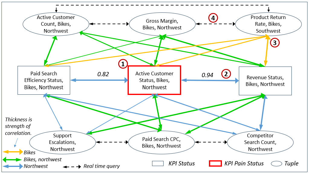
The first three share both Bikes and Northwest. The next three share only one member. That provides a sensible order in which to calculate missing or stale correlations.
The number of shared members is not itself evidence of correlation. It is a candidate-ranking signal, a reason to spend compute testing the relationship. Two tuples sharing several members can be completely uncorrelated, while two tuples from distant domains can be tightly coupled. The TCW exists partly to discover those distant and unexpected relationships.
Nor should every shared member carry the same weight. Product Category = Bikes may be highly informative. All Products, All Customers, or a date range used throughout the enterprise is not. A simple affinity score can therefore weight shared members by specificity:
TupleAffinity(A, B) = sum of weight(m) for each informative member m shared by A and B
The weights could consider:
- Whether the members are exactly the same governed member in the semantic layer or merely have similar labels.
- How frequently the member occurs among candidate tuples.
- Whether the member is a specific leaf-level value or an
All/default member. - Whether the dimension is germane to the seed problem.
- Whether the relationship crosses domains and therefore adds a new analytical perspective.
This resembles the inverse-frequency idea used in information retrieval: a member appearing almost everywhere tells us little, while a rare, specific shared member substantially narrows the context.
Formula and data lineage should also be checked. If two measures are constructed from the same base measure, their high correlation may be a known arithmetic dependency rather than a new empirical discovery. That relationship is still worth representing, but it should be labeled differently. The KPI Status Relationship Graph provides the precedent: common formula elements explain structural relationships among KPIs, while correlations measure how their observed values behave together over time.
It’s important to note that this is even more effective if multiple KPI statuses exhibit pain. That gives us paths to explore.
The Immense Value of a Pre-Aggregated Semantic Layer
The staged protocol reduces the number of candidate pairs. A pre-aggregated semantic layer, such as what is provided by Kyvos Insights, reduces the cost of testing each surviving pair. This is the division of labor described in The Role of OLAP Cubes in Enterprise Intelligence: the semantic layer makes dimensional retrieval fast enough for the graph to materialize and reconstruct selected analytical relationships as needed [5].
Most of the expensive work is not the Pearson formula. It is retrieving and aggregating the underlying facts into two aligned time series. Once the semantic layer returns 52 weekly observations for each tuple, calculating a correlation (such as with Pearson or Spearman) is minor work. The problem becomes manageable when both sides are addressed:
- Probe only candidates that currently have a reason to be examined.
- Retrieve their aggregated histories from a system designed for fast dimensional slicing and dicing.
Pre-aggregation does not magically remove the combinatorial growth of all possible pairwise correlations. It makes selected correlations inexpensive enough to calculate on demand. This permits the TCW to behave more like a cache than a permanently completed graph. Strong and currently valuable edges remain materialized. Weak, old, or rarely used edges can expire because they can be reconstructed with relatively little penalty.
A cached correlation edge needs enough context to determine whether it can safely be reused:
| Edge property | Why it matters |
|---|---|
| Tuple A and Tuple B | Identifies the two qualified measures. |
| Correlation method | Distinguishes Pearson, Spearman, lagged, nonlinear, or other relationships. |
| Correlation value | Records the measured strength and direction. |
| Observation count | Indicates how much evidence participated in the calculation. |
| Date window | Defines the period in which the relationship was observed. |
| Time grain | Distinguishes daily, weekly, monthly, or other comparisons. |
| Lag | Records whether one series was shifted relative to the other. |
| Slice context | Preserves the dimensional qualification of each series. |
| Last calculated | Supports expiration and refresh decisions. |
| Formula/model versions | Identifies the KPI definitions used during calculation. |
Freshness cannot be represented by last calculated alone. A correlation calculated yesterday over ten years of monthly data may still be inappropriate for a problem that emerged during the last six weeks. Compatibility of window, grain, lag, and tuple context matters as much as age.
Round 3: Ask the Insight Space Graph What Happened
A TCW edge says that two qualified measures moved together over a specified period. It does not explain when the meaningful movement occurred, what shape it took, or what else analysts saw around it. This is where the Insight Space Graph becomes the next investigative surface.
The tuples on a promising TCW path can be used to find ISG QueryDef nodes involving the same metrics, members, columns, and time periods. The associated insights may include:
- An inflection where a series moved to a different level and remained there.
- A spike or drop associated with a short-lived event.
- A trend that began before the distressed KPI crossed its threshold.
- A measure that remained stable, providing negative evidence.
- A cluster suggesting that the population contains two different operating conditions.
- A breakpoint or regime change indicating that one global correlation conceals multiple local relationships.
- A composition or ranking change that is not visible in the two time series alone.
Suppose Active Customer Status and Competitor Search Count are strongly inversely correlated. The ISG might show that both series contain inflections during the week of February 11, 2024. Other QueryDefs from that period might show:
- Revenue and customer count began declining.
- Average revenue per remaining customer stayed stable.
- Paid search cost rose sharply.
- A previously insignificant search term entered the top rankings.
- Price, fulfillment time, and support response remained stable.
The correlation identifies a neighborhood. The insights give that neighborhood shape. Inflections are especially valuable because they narrow a long correlation window to a possible boundary where something changed. The Insight Function Array makes these shapes queryable by preserving detected observations together with the QueryDef context that produced them.
Round 4: Let Time Open a Cross-Domain Search
Time provides a common element through which otherwise unrelated tuples can be compared. However, time by itself does not tell the TCW which of the immense number of possible cross-domain relationships should be calculated. Those hints come from the ordinary BI work already taking place across the enterprise.
Analysts in Sales, Marketing, Finance, Customer Success, Operations, Human Resources, and other domains continually investigate problems from their own perspectives. They use the data sources, terminology, measures, and visualizations natural to their work. A sales analyst may be investigating disappearing customers while a marketing analyst studies a rapidly rising search term. A customer-success analyst may be examining cancellation reasons while an operations analyst confirms that fulfillment and service levels remain stable.
These analysts are generally not operating as a coordinated enterprise-wide investigative team. They may not know what analysts in other domains are investigating, and they may not even realize that their respective problems are related. Each analyst sees a small but meaningful portion of the enterprise through the lens of the problem she is trying to resolve.
The main idea of the ISG and TCW is to integrate this distributed analytical work automatically. As described in Insight Function Array: How the Insight Space Graph Notices, Remembers, and Connects, the same dataframe returned to a BI visualization is also passed through the Insight Function Array. The IFA applies functions appropriate for the visualization and data shape, looking for features such as trends, spikes, inflections, stable measures, dominant categories, clusters, outliers, and correlations.
The analyst does not need to explicitly report each observation. She may not notice it, may consider it irrelevant to her immediate problem, or may have no idea who else in the enterprise would find it important. If an insight meets its threshold, the IFA retains it along with its QueryDef: the measures, dimensions, filters, members, source, date range, affected period, detection method, and strength of the result.
The Insight Space Graph turns those temporary query results into persistent, addressable observations. Insights gathered from many analysts, BI tools, domains, data sources, and periods of time become part of one enterprise-wide observation layer. The ISG does not require the analysts to know one another, coordinate their searches, or recognize the larger significance of what they encountered.
This is especially important because an observation can be unimportant within the query that produced it but important in the context of another query. A marketing analyst may see an unfamiliar search term suddenly climb the rankings but have no reason to connect it to lost customers. A customer-success analyst may see “switched to another provider” become a dominant cancellation reason without knowing that Marketing has encountered the name of the new provider. An operations analyst may find nothing unusual, but that stability provides negative evidence against fulfillment, price, or service problems.
As described in Enterprise Intelligence, TL;DR, the ISG and TCW passively capture what many analysts have seen—or could have seen—through their normal BI activity. The value comes from combining analytical attention that would otherwise remain scattered across dashboards, saved reports, departments, and human memories.
The insights retained in the ISG then provide hints about which TCW relationships should be created. A significant inflection lights up the tuples involved in that query. A spike, cluster, ranking change, or stable measure does the same. If insights from different QueryDefs involve the same or nearby periods, that temporal overlap supplies a reason to test their tuples against one another. Shared entities, dimensions, semantic relationships, or data-catalog elements can raise their priority further.
The IFA insight does not assert that two tuples from different queries are correlated. It identifies a promising place to look. The TCW performs the empirical test. Existing compatible correlations can be retrieved, while missing or stale correlations can be calculated through the pre-aggregated semantic layer and materialized when they prove strong enough to retain.
For example, an inflection in Active Customer Status and the sudden rise of an unfamiliar search term might cause the TCW to calculate a relationship between Active Customer Count and searches for that term. A sharp increase in customers reporting that they switched providers supplies another candidate tuple. Stable fulfillment and support measures may produce weak relationships, helping eliminate internal operational explanations. The ISG supplies the scattered observations; the TCW determines which of them move together.
Strong TCW relationships can then lead back to the ISG. The associated QueryDefs reveal what the analysts were examining, which filters they applied, what else appeared in their dataframes, and which other insights occurred nearby. Those details can suggest additional tuples and another round of correlations. The process can continue outward into domains that shared no obvious dimensional members with the original KPI.
This is the deeper reason that time opens a cross-domain search. Analysts throughout the enterprise are continually viewing different parts of the business, often unaware of one another’s work. The IFA notices features in their query results. The ISG remembers and integrates those observations. The TCW uses them as hints for relationships worth testing. Together, they turn many isolated attempts to resolve local problems into a continuing enterprise-wide investigation.
Figure 4 illustrates this widening from the original KPI, through its correlation neighborhood, into the observations accumulated from normal BI work across the enterprise.
- Correlated KPI neighborhood. Beginning with the distressed KPI tuple, the TCW retrieves or calculates its relationships with other KPI tuples. Positive and negative correlations identify KPIs participating in the same disturbance, while weak correlations help eliminate unproductive paths. These relationships guide the investigation; they do not, by themselves, establish causation.
- Tuples sharing semantic members. The probe expands to tuples sharing product, region, customer, organizational, or other governed members with the distressed KPI and its strongest neighbors. The more informative members two tuples share, the higher their initial priority. A pre-aggregated semantic layer makes it practical to retrieve their aligned histories and test correlations quickly.
- ISG insights sharing the inflection period. The Insight Space Graph is searched for trends, spikes, inflections, and other insights discovered during ordinary analyst work that overlap the disturbance period. These insights may have been produced by analysts in different departments who were unaware of the present investigation. Their shared timing provides clues about additional tuples and correlations worth testing.
- Cross-domain tuples with no obvious original overlap. ISG clues can carry the investigation into domains that share no product, region, customer, or other obvious member with the starting tuple. An independently discovered inflection may nominate an otherwise unexpected pair, causing the TCW to create or refresh its correlation. Strong relationships open new investigative paths; weak ones provide negative evidence and help narrow the remaining hypotheses.

Casting a Wide Net
The rounds described so far might sound like a process for keeping the search close to a misbehaving KPI. That is how the investigation begins, but it is not the larger purpose of the TCW. The KPI tells us where to cast the net. From there, the net should spread far enough to discover relationships that no analyst would have thought to request individually.
Much of the intuition behind the TCW comes from Map Rock, particularly the Correlation Grid described in Map Rock—10th Anniversary and Some Data Mesh Talk. The rows and columns of the grid were each generated by an MDX query. Each axis could specify a cube, measure, dimensional members, slicers, and a date range. The cells of the grid displayed the correlations between the tuples produced by the two axes.
Instead of asking about one relationship at a time, the user could place one population of tuples on the rows, another population on the columns, and examine the resulting field of correlations. A Finance cube could be compared with a Customer cube, a Customer cube with an Inventory cube, or product categories with countries. Date provided the common axis over which the tuples could be compared, even when the cubes had no customer, product, or location dimensions in common.
That was the meaning of “casting a wide net.” The power was not in any one Pearson correlation. It was in generating many candidate relationships at once, quickly enough for the analyst to slice, dice, change the axes, and try again without losing the train of thought. Correlations selected by the analyst were saved, along with unselected correlations that appeared significant. Those relationships could then be connected through their common elements into what I called “Pearson Networks of Correlation.”
Casting this kind of wide net is predicated on fast query retrieval. Calculating the Pearson coefficient after two aligned arrays have been retrieved is inexpensive. The costly part is repeatedly locating, filtering, aggregating, and aligning the underlying data for all the tuples placed on the two axes. If every new cast requires long scans of detailed source data, exploration slows to the point where the analyst loses the train of thought and the TCW cannot probe a large candidate population economically.
This is why the semantic layer is fundamental to the TCW. It provides the governed measures, dimensional members, hierarchies, calculations, and date grains from which tuples are constructed. It also provides the consistent definitions needed to compare tuples from different queries and domains. A wide net is not valuable if Revenue, Customer, or Northwest silently means something different on each side of the correlation.
A pre-aggregated semantic layer adds the required speed. Kyvos is designed to combine a governed semantic model with smart aggregation and caching so that multidimensional queries can be returned at interactive speed, even across very large data volumes. The aggregates are created once and reused across many queries. That is especially important to the TCW, which may request many variations of the same measures across different members, date ranges, and grains while progressively widening an investigation.
The TCW carries the Map Rock idea beyond the session-oriented Correlation Grid. It turns relationships discovered through many explorations into a persistent web. A relationship noticed while investigating a customer problem can later become relevant to an inventory problem, even though the second analyst never saw the original query. What began as a wide-net search becomes enterprise memory.
However, casting a wide net does not mean blindly calculating every possible correlation in the enterprise. That would produce a cross-join of an immense tuple space. KPI-first probing provides a way to cast the net progressively. The first throw covers the other KPI tuples. The next expands through shared tuple elements. ISG insights then expose inflection periods and other contexts that can carry the search into domains with no obvious relationship to the original KPI.
The net is therefore wide in reach but directed in where it begins. Current pain, analyst activity, previously discovered insights, common tuple elements, and unusual changes determine where the next portion of correlation space should be examined. The semantic layer gives those tuples consistent meaning, while the pre-aggregated performance of a platform such as Kyvos makes repeated casting fast enough to sustain exploration. The TCW retains the relationships worth remembering.
Map Rock supplied the original wide-net mechanism. The fast semantic layer makes it possible at enterprise scale. The TCW makes it continuous, selective, and cumulative.
The ISG and TCW Form a Feedback Loop
The usual description of their relationship begins with BI activity. Analysts issue queries, the IFA detects noteworthy features in the resulting dataframes, and those findings are stored in the ISG. Tuples emphasized by the queries and insights become candidates for correlation in the TCW.
That remains true, but it is only half of the interaction.
Once a TCW path becomes relevant, its tuples can be used to search the ISG for prior analytical observations. Those observations can expose inflection dates, overlooked dimensions, candidate confounders, negative evidence, and other tuples. The newly discovered tuples are then sent back to the TCW for another round of correlation testing.
The loop is illustrated in Figure 5.
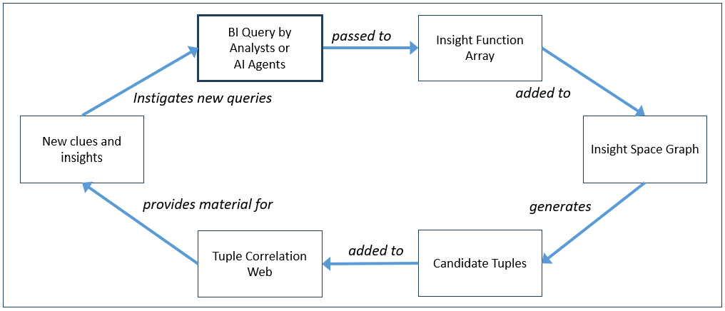
The process is exploratory without being indiscriminate. Each round is justified by evidence found in the prior round.
A Concrete Probing Procedure
The KPI-first extension can be summarized as the following procedure:
- Select the seed tuple. A KPI status crosses a pain threshold, deteriorates unusually quickly, or otherwise demands attention. Preserve its complete dimensional qualification.
- Choose the comparison context. Specify the date window, time grain, acceptable missing-data behavior, and initial correlation method.
- Probe the KPI neighborhood. Correlate the seed against compatible KPI-status tuples. Reuse only edges calculated with compatible context and sufficiently current model versions.
- Validate promising KPI relationships. Compare raw values as well as statuses when possible. Examine negative correlations, lags, sample size, and obvious formula dependencies.
- Rank shared-member candidates. Gather non-KPI tuples sharing informative members with the seed and its strongest KPI neighbors. Weight specific members more heavily than ubiquitous defaults.
- Calculate missing or stale correlations. Retrieve aligned time series from the pre-aggregated semantic layer and materialize only the relationships that meet retention criteria.
- Search the ISG. Find QueryDefs and insights involving the correlated tuples. Pay particular attention to coincident or ordered inflections, spikes, stability, clusters, and regime changes.
- Promote time-local clues. Treat a shared inflection period as a temporary investigative anchor. Find other insights and tuples active during that period even when they do not share the original dimensional members.
- Repeat with a wider neighborhood. Submit the new tuples to the TCW while retaining the original problem context and a path back to the distressed KPI.
- Escalate the surviving paths. Present the strongest, most coherent chains as hypothesis material for analysts, subject-matter experts, System 1 functions, or System 2 reasoning.
The result is not a declaration of cause. It is an evidence-ranked map of where to investigate next.
Guardrails
The staged search makes the TCW more tractable, but it does not make correlation safe from careless interpretation.
- Align the series Two tuples should be compared at compatible grains and over meaningful overlapping windows. A daily operational KPI and a quarterly financial KPI cannot be correlated merely by placing their available values into two arrays. Missing periods, late-arriving facts, and differences in business calendars must be handled explicitly.
- Preserve KPI history KPI targets, tolerances, formulas, and dimensional definitions change. Historical statuses must either be stored as facts or reproducible from versioned definitions. Otherwise, recalculation silently applies today’s intentions to yesterday’s conditions.
- Distinguish discovery from arithmetic Two KPIs may correlate because one formula includes the other. That is a structural dependency, not an independently discovered relationship. The Data Catalog and formula lineage should label it accordingly.
- Control repeated testing Even a narrowed candidate population can produce coincidental high correlations. Sample size, repeated-testing controls, holdout periods, persistence, and validation across alternative windows should influence whether an edge is retained or promoted.
- Do not stop at Pearson Relationships can contain lags, thresholds, multiple regimes, and reversals that collapse into an unimpressive global Pearson score. Pearson is a good inexpensive scout, not the final judge.
- Do not remain trapped among shared members Shared tuple elements provide an efficient second round, but the most valuable TCW discovery may connect domains with no obvious dimensional overlap. The ISG’s inflection dates, semantic links, analyst activity, embeddings, and wider probing mechanisms provide the bridges into that territory.
What This Adds to the TCW Probing Protocol
The original TCW Probing Protocol explains why the entire correlation space cannot be materialized and identifies the signals that should receive attention. This extension adds a repeatable traversal order:
- Pain first.
- Then the other KPIs.
- Then nearby tuples sharing business context.
- Then the ISG observations surrounding the strongest relationships.
- Then outward through the time and meaning exposed by those observations.
Starting with KPIs is not merely a computational optimization. KPIs express what the enterprise has already decided matters. Their status functions translate raw measures into the distance between what is happening and what was intended. When one enters pain, it supplies both a reason to investigate and a qualified coordinate from which the investigation can begin.
Shared tuple members keep the early search close to that coordinate. Correlations determine which of those nearby possibilities have empirical support. ISG insights reveal where the behavior changed and what else was visible around that change. Those discoveries then provide the next set of coordinates.
Pruning
Tuple correlations do not all need to remain in the hot TCW indefinitely. Pruning can move them to cold storage based on time-to-live, use count, time since last use, correlation strength, current investigative relevance, or the cost of recalculating them. Pruning is therefore not necessarily deletion. It removes a tuple or correlation from the active working graph while preserving enough information to recover it.
Date ranges can also be divided between storage tiers. For example, an older closed range such as [Begin of Time, 2025-12-31] might be archived while [2026-01-01, Today] remains hot. The older aggregated series, correlation state, and calculation provenance can be retrieved when an investigation requests the longer range.
A structure similar to a Data Vault Point-in-Time (PIT) table could support this. A PIT-like TCW structure would record the tuple or correlation identifier, date range, as-of date, formula and semantic-model versions, storage tier, and the location of the corresponding artifact. It would act as a small temporal index into the hot and cold portions of the TCW. This follows the Data Vault use of a PIT table to locate the historical records applicable at a particular point in time.
When an archived relationship becomes relevant again, the TCW can rehydrate it. If the archived calculation has the required date range, grain, method, and formula versions, it can be reused. Otherwise, the pre-aggregated semantic layer can recalculate it. In this way, pruning keeps the active TCW manageable without forcing the enterprise to forget relationships it has already observed.
My Related Blogs
- Tuple Correlation Web Probing Protocol. The protocol extended by this article, including KPI distress, tuple illumination, prioritization, signal half-life, and dynamic materialization of the TCW.
- Insight Space Graph. See especially “Correlating Status Metrics of Key Performance Indicators”, which discusses quickly calculating KPI statuses across tuples and forming chains of KPI-status correlations.
- The Effect Correlation Score for KPIs. Discusses status-to-status versus value-to-value correlation, historical KPI values, periodic revalidation, grain, seasonality, and calculation cost.
- KPI Status Relationship Graph Revisited with LLMs. Relates KPIs through common formula and source elements and distinguishes structural formula relationships from empirical KPI-status correlations.
- The Role of OLAP Cubes in Enterprise Intelligence. Explains how pre-aggregation supports fast ISG/TCW querying and inexpensive reconstruction of pruned analytical artifacts.
- Insight Function Array: How the Insight Space Graph Notices, Remembers, and Connects. Describes how ordinary BI dataframes are examined for inflections, spikes, trends, clusters, correlations, stable measures, and other insights retained with QueryDef context.
- Explorer Subgraph: The Dynamic Cartography of Relation Space. Places ISG and TCW probing in a wider feedback loop and treats BI queries as attention signals.
- Correlation Is a Hint Towards Causation. Discusses stress-testing correlations, confounding variables, and the use of correlation chains as material for a larger explanatory story.
- Chains of Unstable Correlations. Extends TCW edges beyond global linear correlation to thresholds, hockey sticks, regime changes, and other nonlinear relationships.
- The Complex Game of Planning. Discusses KPI pain, KPI snapshots, correlations, inflections, and the role of changing system attributes in planning.
- An MDX Primer. Background on tuples, partial tuples, default members, slicer context, and multidimensional analytical space.


One thought on “KPI-First Probing of the Tuple Correlation Web”